Chapter 4 Performing spatial operations in R

By now you have come a long way in terms of taking your spatial data, and visualising it using maps, and being able to present the values of a variable using thematic maps. You have had some practice in taking data which has a spatial component, and joining it to a shapefile, using the common column, in order to be able to visually demonstrate variation on something, such as the crime rate, across space.

We hope that you are finding this to be really exciting stuff, and an opportunity to get yourselves accustomed to spatial data. If there is anything you are unsure about, or want to catch up on, please do not hesitate to revisit older material, and ask the teaching staff questions about it. We build on each week acquiring knowledge cumulatively, so don’t let yourself get stuck anywhere down the line. But, if you’re ready, today we will go a step further, and get your hands dirty with spatial manipulation of your data.

Thus far, our data manipulation exercises were such that you might be familiar with, from your earlier exposures to data analysis. Linking datasets using a common column, calculating a new variable (new column) from values of existing variables, these are all tasks which you can perform on spatial or non-spatial data. However today we will explore some exercises in data manipulation which are specific to spatial data analysis. After this session you can truly say you are masters of spatial data manipulation. So let’s get started with that!

The main objectives for this session are that by the end you will have:

used geocoding methods to translate postcodes into geographic coordinates
made interactive point map with leaflet
met a new format of spatial shape file called geojson
subset points that are within a certain area using a spatial operation
created new polygons by generating buffers around points
counted the number of points that fall within a polygon, known as points in polygon

These are all very useful tools for the spatial crime analyst, and we will hope to demonstrate this by working through an example project, where you would make use of all of these tools.

The packages we will use today are:

dplyr
janitor
leaflet
readr
tidygeocoder
sf

4.1 Criminality of place

Let’s consider the assumption that licenced premises which serve alcohol are associated with increased crimes. We might have some hypotheses about why this may be.

One theory might be that some of these serve as crime attractors.

Crime attractors are particular places, areas, neighbourhoods, districts which create well-known criminal opportunities to which strongly motivated, intending criminal offenders are attracted because of the known opportunities for particular types of crime. Examples might include bar districts; prostitution areas; drug markets; large shopping malls, particularly those near major public transit exchanges; large, insecure parking lots in business or commercial areas. The intending offender goes to rough bars looking for fights or other kinds of ‘action’.

On the other hand, it is possible that these areas are crime generators.

Crime generators are particular areas to which large numbers of people are attracted for reasons unrelated to any particular level of criminal motivation they might have or to any particular crime they might end up committing. Typical examples might include shopping precincts; entertainment districts; office concentrations; or sports stadiums.

To read further in crime attractors vs crime generators turn to your recommended reading of Brantingham, P., & Brantingham, P. (1995). Criminality of place. European journal on criminal policy and research, 3(3), 5-26.). There have since been more developments, for example about crime radiators and absorbers as well (watch this Risky Places lecture from Kate Bowers: to learn more!

It’s possible that some licensed premises attract crimes, due to their reputation. However it is also possible that some of them are simply located in areas that are busy, attracts lots of people for lots of reasons, and crimes occurr as a result of an abundance of opportunities instead.

In any case, what we want to do is to examine whether certain outlets have more crimes near them than others. We can do this using open data, some R code, and spatial operations.

4.2 Spatial operations

Spatial operations are a vital part of geocomputation. Spatial objects can be modified in a multitude of ways based on their location and shape. For a comprehensive overview of spatial operations in R I would recommend the relevant chatper Chapter 4: Spatial Operations from the project of Robin Lovelace and Jakub Nowosad, Geocomputation with R.

Spatial operations differ from non-spatial operations in some ways. To illustrate the point, imagine you are researching road safety. Spatial joins can be used to find road speed limits related with administrative zones, even when no zone ID is provided. But this raises the question: should the road completely fall inside a zone for its values to be joined? Or is simply crossing or being within a certain distance sufficent? When posing such questions it becomes apparent that spatial operations differ substantially from attribute operations on data frames: the type of spatial relationship between objects must be considered.(Lovelace & Nowosad, 2018)

So you can see we can do exciting spatial operations with our spatial data, which we cannot with the non-spatial stuff. Let’s get to it!

4.3 Download some boundary data for relevant wards

When considering the areas of interest for these sorts of crimes, you may hear people refer to the “night time economy” problem. This refers to the fact that many of these crimes occur during the night, when people are out socialising, drinking, and generally having a good time. The night time economy is an important part of many cities, but it also brings with it challenges in terms of crime and disorder. When we consider what area to study for night time economy, you need to have some understanding of the place of interest. For example, in Manchester you might want to consider Deansgate and Piccadilly areas where many bars and pubs are situated.

To study these areas, we try a different unit of analysis from LSOAs, specifically we will look at wards. These are larger, administrative units, and in this case reflect the different land use - specifically we can select Deansgate and Piccadilly wards.

To get these data we will go back to the ONS Boundary Data Selector tool which we used in week 2. Follow the steps for selecting your desired geography and areas again, but this time select England > North West > Manchester, and choose Deansgate and Piccadilly:

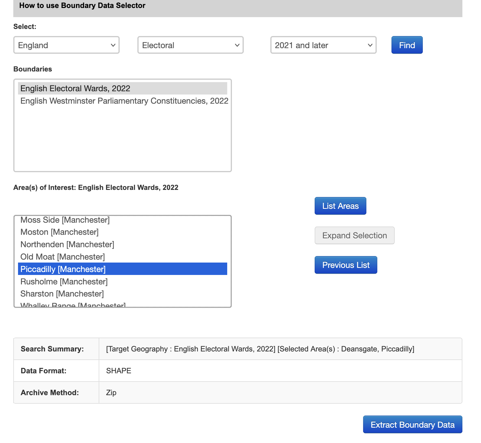When you click on Extract Boundary data you will be shown the same result and you must download the .zip folder like you did in week 2, extract it, and save the contents to your data folder. Once again you are going to load in a shapefile using the st_read() function.

central_wards <- st_read("data/BoundaryData/deansgate_picc_wd_2022.shp")

## Reading layer `deansgate_picc_wd_2022' from data source 
##   `/Users/user/Desktop/resquant/crime_mapping_textbook/data/BoundaryData/deansgate_picc_wd_2022.shp' 
##   using driver `ESRI Shapefile'
## Simple feature collection with 2 features and 5 fields
## Geometry type: POLYGON
## Dimension:     XY
## Bounding box:  xmin: 382619.4 ymin: 397083 xmax: 385703.7 ymax: 399529.9
## Projected CRS: OSGB36 / British National Grid

Let’s have a look

ggplot() + 
   annotation_map_tile() +  # add basemap
  geom_sf(data = central_wards)

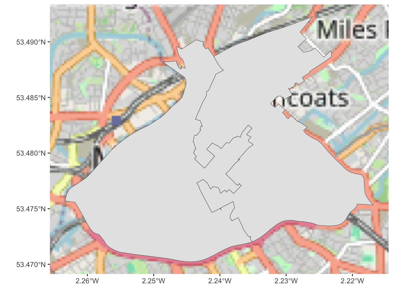Right, we now have these two wards to cover the area of city centre manchester, which we consider to be our main focus for the following work on the night time economy.

4.4 Activity 1: First spatial operation: union

So let’s unite these two into one boundary. To do this, we will perform our first spatial operation, a spatial union! We use the st_union() function from the sf package.

# create new boundary, called manchester_ward by union these two

city_centre <- st_union(central_wards)

And now we have a single polygon whic covers the whole of the city centre. We can plot it to see:

ggplot() + 
   annotation_map_tile() +  # add basemap
  geom_sf(data = city_centre)

## Zoom: 12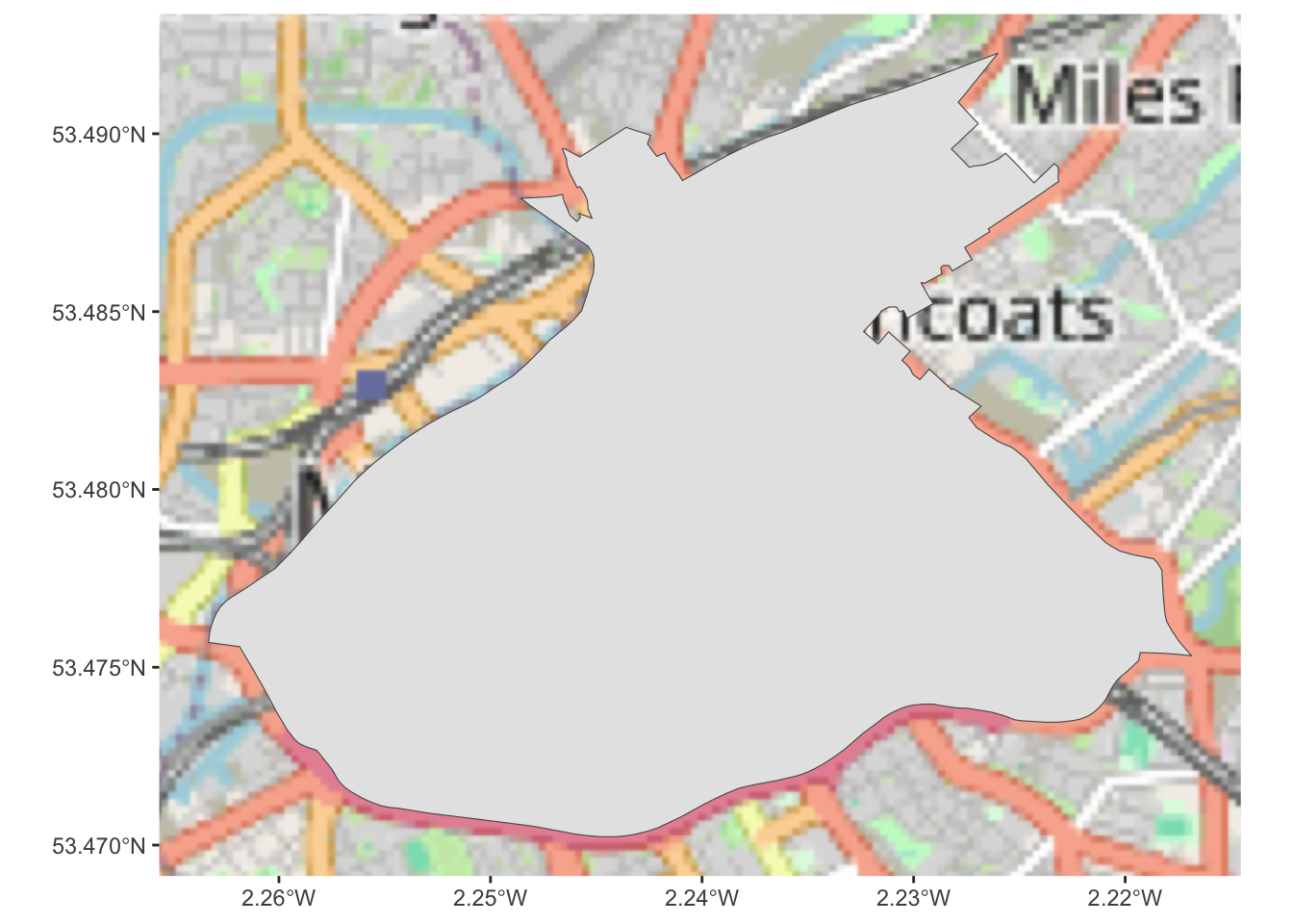

You can see the boundary down the middle is gone, and we have only 1 item here, whereas we had 2 in the previous (separaet deansgate and piccadilly). Great, our first spatial operation is complete, and that was not too difficult. We now have a spatial boundary for city centre Manchester.

Now before we move on to get more data, I want to save this output. But I don’t want to keep generating so many files like we do with the shapefile format. So instead, we will now introduce another spatial file format: geojson.

4.4.1 Meet a new format of shapefile: geojson

GeoJSON is an open standard format designed for representing simple geographical features, along with their non-spatial attributes. It is based on JSON, the JavaScript Object Notation. It is a format for encoding a variety of geographic data structures.

Geometries are shapes. All simple geometries in GeoJSON consist of a type and a collection of coordinates. The features include points (therefore addresses and locations), line strings (therefore streets, highways and boundaries), polygons (countries, provinces, tracts of land), and multi-part collections of these types. GeoJSON features need not represent entities of the physical world only; mobile routing and navigation apps, for example, might describe their service coverage using GeoJSON.

To tinker with GeoJSON and see how it relates to geographical features, try geojson.io, a tool that shows code and visual representation in two panes.

To save our city centre boundary as a geojson file, we can use the st_write() function:

st_write(city_centre, "data/mcr_city_centre.geojson")

And then whenever we want to import it we use the st_read() function again.

city_centre <- st_read("data/mcr_city_centre.geojson")

The advantages of geojson files over shapefiles is that they are a single file (shapefiles are made up of multiple files), they are text based and so can be easily read in and written out using web services, and they are more lightweight than shapefiles.

4.5 Getting open data from the city

Manchester City Council have an Open Data Catalogue on their website, which you can use to browse through what sorts of data they release to the public. There are some more and some less interesting data sets made available here. It’s not quite as impressive as the open data from some of the cities in the US such as New York or Dallas but we’ll take it.

One interesting data set, especially for our questions about the different alcohol outlets is the Licensed Premises data set. This details all the currently active licenced premises in Manchester. You can see there is a link to download now.

Have a look at the terms and conditions for using these data once again. They are published under an Open Government Licence and so you must acknowledge the source of the data in any publication or application you make using this data. You can include the statement: Contains public sector information licensed under the Open Government Licence v3.0. for example in the caption of any figures or maps that you make with these data

As always, there are a few ways you can download this data set. On the manual side of things, you can simply right click on the download link from the website, save it to your computer, and read it in from there, by specifying the file path. Remember, if you save it in your working directory, then you just need to specify the file name, as the working directory folder is where R will first look for this file.

So without dragging this on any further, let’s read in the licensed premises data directly from the web:

lic_prem <- read_csv("http://www.manchester.gov.uk/open/download/downloads/id/169/licensed_premises.csv")

## Warning: One or more parsing issues, call `problems()` on your
## data frame for details, e.g.:
##   dat <- vroom(...)
##   problems(dat)

## Rows: 65535 Columns: 36
## ── Column specification ────────────────────────────────
## Delimiter: ","
## chr (23): EXTRACTDATE, ORGANISATIONURI, ORGANISATIONLABEL, CASEDATE, SERVICE...
## dbl  (1): CASEREFERENCE
## lgl (12): LATENIGHTREFRESHMENT, ALCOHOLSUPPLY, OPENINGHOURS, LICENCEENDDATE,...
## 
## ℹ Use `spec()` to retrieve the full column specification for this data.
## ℹ Specify the column types or set `show_col_types = FALSE` to quiet this message.

You can always check if this worked by looking to your global environment on the right hand side and seeing if this ‘lic_prem’ object has appeared. If it has, you should see it has 65535 observations (rows), and 36 variables (columns).

Let’s stop for a minute. Sure Manchester is not small. But 65,535 licenced premises would be a bit wild. Let’s have a look at what this data set looks like. You can use the View() function for this:

View(lic_prem)

We can see there are some interesting and perhaps less interesting columns in there. And if we scroll down we can see many many empty rows (where all values are NA). Let’s get rid of these:

# remove all rows where every value is NA
lic_prem <- lic_prem %>%
  filter(!if_all(everything(), is.na))

Now we end up with only 2265 observations. Much more reasonable!

As we are interested in venues that serve alcohol, we can further remove the ones where the value for the variable ALCOHOLSUPPLY is FALSE.

# keep only rows where ALCOHOLSUPPLY is TRUE
lic_prem <- lic_prem %>%
  filter(ALCOHOLSUPPLY == TRUE)

This leaves us with 1918 venues where alcohol is served who are licenced by Manchester City Council. Now if we have a look at the data, we see that there is no geometry associated with this dataset. No latitude longitude columns either for us to work with. What we do have though, is addresses.

4.6 What is geocoding and how can we use addresses to put venues on the map?

Geocoding is the process of converting place descriptions, such as street addresses or place names, into geographic coordinates (latitude and longitude), while reverse geocoding does the opposite (translates coordinates into addresses). It works by sending these inputs to a geocoding service, which matches them against spatial databases and returns the best geographic estimate. The R package tidygeocoder provides a simple, consistent way to access several of these services within a tidy data workflow. You supply address or coordinate columns from a data frame, choose a service, and tidygeocoder handles batching, duplicates, and rate limits automatically, returning the results as a tidy tibble that can be directly mapped, analysed, or joined to other spatial data.

Let’s illustrate with an example:

# load the package
library(tidygeocoder)

# create a new dataframe which has coordinates saved into columns lat and long
lat_longs <- lic_prem %>% head() %>%  # here we take the first 6 observations from our data - this is for saving time
  mutate(addr = paste(LOCATIONTEXT,  # create a new column that pastes together the address,
                      POSTCODE,      # the postcode and 
                      "Manchester, UK", # appends Manchester, UK to the end of it
                      sep = ", ")) %>% 
  geocode(addr,   # use geocode function on newly created column
          method = 'osm', # use open street map method
          lat = latitude , long = longitude) # name resulting columns

So above we first take only the first 6 venues from our data. This is only to save time here in the lab. The geocoding using this approach takes about 1 second per address, so with the ~2,000 venues that should be around half an hour. We don’t want to wait so long just now, so instead here we take the first 6 cases. I will show a more targeted way to filter in a minute.

Then we create a variable that combines all the address information from the dataframe. There are 2 columns, address (in column LOCATIONTEXT) and post code (in column POSTCODE). We paste these together and append “Manchester, UK” to the end of it, so that the geocoding service knows we are looking for addresses in Manchester.

Finally we use the geocode() function from the tidygeocoder package to geocode this address. We specify which column has the address information (the one we just created), which geocoding method to use (in this case open street map, which is free), and finally we specify what to call the resulting latitude and longitude columns.

You can have a look at the resulting dataframe and you will see there are now latitudes and longitudes for these 6 venues. We can use these to put them on the map.

But let’s think of a more targeted way to filter venues before we move on to mapping these.

4.6.1 Activity 2: Subsetting using pattern matching

We could use spatial operations here, and geocode all the postcodes at this point, then use a spatial file of city centre to select only the points contained in this area. The only reason we’re not doing this is because the geocode function takes a bit of time to geocode each address. As I mentioned above, it would only be about 30 minutes, but we don’t want to leave you sitting around in the lab for this long, so instead we will try to subset the data using pattern matching in text. In particular we will be using the grepl() function. This function takes a pattern and looks for it in some text. If it finds the pattern, it returns TRUE, and if it does not, it returns FALSE. So you have to pass two parameters to the grepl() function, one of them being the pattern that you want it to look for, and the other being the object in which to search.

So for example, if we have an object that is some text, and we want to find if it contains the letter “a”, we would pass those inside the grepl() function, which would tell us TRUE (yes it’s there) or FALSE (no it’s not there):

#example 1: some_text with 'a'
some_text <- "this is some text that has some letter 'a's"
grepl("a", some_text)

## [1] TRUE

You can see this returns TRUE, because there is at least one occurrence of the letter a. If there wasn’t, we’d get FALSE:

#example 2: some_text without 'a'
some_text <- "this is some text tht h_s some letter '_'s"
grepl("a", some_text)

## [1] FALSE

4.6.2 Activity 3: Pattern matching to find city centre premises

So we can use grepl(), to select all the cases where we find the pattern “M1” in the postcode. NOTICE the space in our search pattern. It’s not “M1” it’s “M1 ”. Can you guess why?

Well, M1 will be found in M1 but also in M13, which is the University of Manchester’s postcode, and not the part of city centre in which we are interested.

So let’s subset our data by creating a new object city_centre_prems, and using the piping (%>%) and filter() functions from the dplyr package:

#create the city_centre_prems object:
city_centre_prems <- lic_prem %>%
  filter(grepl("M1 ", POSTCODE) )

Now we only have 314 observations (see your global environment), which is a much more manageable number.

4.7 Geocoding from an address

So let’s go back to the geocoding now. We can now use the same approach as above, but this time on our city_centre_prems data frame, which only has the venues in the city centre.

city_centre_prems <- city_centre_prems %>%
  mutate(addr = paste(LOCATIONTEXT,
                      POSTCODE,
                      "Manchester, UK",
                      sep = ", ")) %>%
  geocode(addr,
          method = 'osm',
          lat = latitude , long = longitude)

Be patient, this will take a while, each address has to be referenced against their database and the relevant coordinates extracted. For each point you will see a note appear in red, and while R is working you will see the red stop sign on the top right corner of the Console window.

Also think about how incredibly fast and easy this actually is, if you consider a potential alternative where you have to manually find some coordinates for each address. That sounds pretty awful, doesn’t it? Compared to that, setting the above functions running, and stepping away to make a cup of tea is really a pretty excellent alternative, no?

Right so hopefully that is done now, and you can have a look at your data again to see what this new column looks like. Remember you can use the View() function to make your data appear in this screen.

View(city_centre_prems)

And now we have a column called longitude for longitude and a column called latitude for latitude. Neat! I know there was a lot in there, so don’t worry about asking lots of questions on this!

Another thing you might notice is many NAs:

sum(is.na(city_centre_prems$latitude))

## [1] 107

Out of 353 venues, 107 could not be geocoded. This is likely down to incomplete or incorrect address information. In a real world scenario you would want to go back and check these addresses, perhaps try to manually geocode them, or use another geocoding service to see if you can get better results. But for now we will move on just excluding these venues.

4.8 Making interactive maps with leaflet

Thus far we have explored a few approaches to making maps. We made great use of the tmaps package for example in the past few weeks. But now, we are going to step up our game, and introduce Leaflet as one way to easily make some neat maps. It is the leading open-source JavaScript library for mobile-friendly interactive maps. It is very most popular, used by websites ranging from The New York Times and The Washington Post to GitHub and Flickr, as well as GIS specialists like OpenStreetMap, Mapbox, and CartoDB, some of who’s names you’ll recognise from the various basemaps we played with in previous labs.

In this section of the lab we will learn how to make really flashy looking maps using leaflet. If you haven’t already, you will need to have installed and loaded the leaflet and RColorBrewer packages.

4.8.1 Activity 4: Making an interactive map

You create a map with this simple bit of code:

m <- leaflet() %>%
  addTiles()

And just print it:

Not a super useful map, definitely won’t win map of the week, but it was really easy to make!

You might of course want to add some content to your map.

4.8.1.1 Adding points manually

You can add a point manually:

m <- leaflet() %>%
  addTiles()  %>% 
  addMarkers(lng=-2.230899, lat=53.464987, popup="burglary")
m

Or many points manually, with some popup text as well:

latitudes = c(53.464987, 53.472726, 53.466649) 
longitudes = c(-2.230899, -2.245481, -2.243421) 
popups = c("burglary", "robbery", "stop and search")
df = data.frame(latitudes, longitudes, popups)      

map_practice <- leaflet(data = df) %>%
  addTiles()  %>%  
  addMarkers(lng=~longitudes, lat=~latitudes, popup=~popups)
map_practice

4.8.1.2 Adding data

Last time around we added crime data to our map. In this case, we want to be mapping our licensed premises in the city centre, right? So let’s do this:

city_centre_prems$latitude <- as.numeric(city_centre_prems$latitude)
city_centre_prems$longitude <- as.numeric(city_centre_prems$longitude)

mcr_map <- leaflet(data = city_centre_prems) %>%
  addTiles() %>%
  addMarkers(~longitude, ~latitude, popup = ~paste("Longitude: ", longitude, ", Latitude: ", latitude))

## Warning in validateCoords(lng, lat, funcName): Data contains 107 rows with
## either missing or invalid lat/lon values and will be ignored

mcr_map

You can see that the points are sort of off to one side. Since we subset earlier only those venues who’s postcodes start with “M1” we actually are missing quite a few other places (many Deansgate venues will me M4 or M3). If you were doing a full and proper problem profile of the night time economy in Manchester, you would want to wait the full time and geocode all the venues, and then use the boundary to select only those what are inside the area of interest, rather than shortcuts with the postcode text.

Now let’s say you wanted to save this map. You can do this by clicking on the export button at the top of the plot viewer, and choose the Save as Webpage option saving this as a .html file:

Then you can open this file with any type of web browser (safari, firefox, chrome) and share your map that way. You can send this to your friends not on this course, and make them jealous of your fancy map making skills.

One thing you might have noticed is that we still have some points that are not in Manchester. This should illustrate that the pattern matching approach is really just a work-around. Instead, what we really should be doing to subset our data spatially is to use spatial operations. So now we’ll learn how to do some of these in the next section.

4.8.2 Coordinate reference systems revisited

One important note before we begin to do this brings us back to some of the learning from the second session on map projections and coordinate reference systems, like we discussed in the lecture today. We spoke about all the ways of flattening out the earth, and ways of making sense what that means for the maps, and also how to be able to point to specific locations within these. The latter refers to the Coordinate Reference System or CRS the most common ones we will use are WGS84 and British National Grid.

So why are we talking about this?

It is important to note that spatial operations that use two spatial objects rely on both objects having the same coordinate reference system

If we are looking to carry out operations that involve two different spatial objects, they need to have the same CRS!!! Funky weird things happen when this condition is not met, so beware!

So how do we know what CRS our spatial objects are? Well the sf package contains a handy function called st_crs() which let’s us check. All you need to pass into the brackets of this function is the name of the object you want to know the CRS of.

So let’s check what is the CRS of our licenced premises:

st_crs(city_centre_prems)

## Coordinate Reference System: NA

You can see that we get the CRS returned as NA. Can you think of why? Have we made this into a spatial object? Or is this merely a dataframe with a latitude and longitude column? The answer is really in the question here.

So we need to convert this to a sf object, or a spatial object, and make sure that R knows that the latitude and the longitude columns are, in fact, coordinates.

In the st_as_sf() function we specify what we are transforming (the name of our dataframe), the column names that have the coordinates in them (longitude and latitude), the CRS we are using (4326 is the code for WGS 84, which is the CRS that uses latitude and longitude coordinates (remember BNG uses Easting and Northing)), and finally agr, the attribute-geometry-relationship, specifies for each non-geometry attribute column how it relates to the geometry, and can have one of following values: “constant”, “aggregate”, “identity”. “constant” is used for attributes that are constant throughout the geometry (e.g. land use), “aggregate” where the attribute is an aggregate value over the geometry (e.g. population density or population count), “identity” when the attributes uniquely identifies the geometry of particular “thing”, such as a building ID or a city name. The default value, NA_agr_, implies we don’t know.

cc_spatial <- st_as_sf(city_centre_prems, coords = c("longitude", "latitude"), 
                 crs = 4326, agr = "constant", na.fail = FALSE)

Now let’s check the CRS of this spatial version of our licensed premises:

st_crs(cc_spatial)

## Coordinate Reference System:
##   User input: EPSG:4326 
##   wkt:
## GEOGCRS["WGS 84",
##     ENSEMBLE["World Geodetic System 1984 ensemble",
##         MEMBER["World Geodetic System 1984 (Transit)"],
##         MEMBER["World Geodetic System 1984 (G730)"],
##         MEMBER["World Geodetic System 1984 (G873)"],
##         MEMBER["World Geodetic System 1984 (G1150)"],
##         MEMBER["World Geodetic System 1984 (G1674)"],
##         MEMBER["World Geodetic System 1984 (G1762)"],
##         MEMBER["World Geodetic System 1984 (G2139)"],
##         MEMBER["World Geodetic System 1984 (G2296)"],
##         ELLIPSOID["WGS 84",6378137,298.257223563,
##             LENGTHUNIT["metre",1]],
##         ENSEMBLEACCURACY[2.0]],
##     PRIMEM["Greenwich",0,
##         ANGLEUNIT["degree",0.0174532925199433]],
##     CS[ellipsoidal,2],
##         AXIS["geodetic latitude (Lat)",north,
##             ORDER[1],
##             ANGLEUNIT["degree",0.0174532925199433]],
##         AXIS["geodetic longitude (Lon)",east,
##             ORDER[2],
##             ANGLEUNIT["degree",0.0174532925199433]],
##     USAGE[
##         SCOPE["Horizontal component of 3D system."],
##         AREA["World."],
##         BBOX[-90,-180,90,180]],
##     ID["EPSG",4326]]

We can now see that we have this coordinate system as WGS84. We need to then make sure that any other spatial object with which we want to perform spatial operations is also in the same CRS.

4.8.3 Activity 5: Subset points to those within a polygon

So we have our polygon, our spatial file of the city centre ward. We now want to subset our point data, the cc_spatial data, which has points representing licensed premises.

First things first, we check whether they have the same crs.

st_crs(city_centre) == st_crs(cc_spatial)

## [1] FALSE

Uh oh! They do not! So what can we do? Well we already know that cc_spatial is in WGS 84, because we made it so a little bit earlier. What about this new city_centre polygon?

st_crs(city_centre)

## Coordinate Reference System:
##   User input: OSGB36 / British National Grid 
##   wkt:
## PROJCRS["OSGB36 / British National Grid",
##     BASEGEOGCRS["OSGB36",
##         DATUM["Ordnance Survey of Great Britain 1936",
##             ELLIPSOID["Airy 1830",6377563.396,299.3249646,
##                 LENGTHUNIT["metre",1]]],
##         PRIMEM["Greenwich",0,
##             ANGLEUNIT["degree",0.0174532925199433]],
##         ID["EPSG",4277]],
##     CONVERSION["British National Grid",
##         METHOD["Transverse Mercator",
##             ID["EPSG",9807]],
##         PARAMETER["Latitude of natural origin",49,
##             ANGLEUNIT["degree",0.0174532925199433],
##             ID["EPSG",8801]],
##         PARAMETER["Longitude of natural origin",-2,
##             ANGLEUNIT["degree",0.0174532925199433],
##             ID["EPSG",8802]],
##         PARAMETER["Scale factor at natural origin",0.9996012717,
##             SCALEUNIT["unity",1],
##             ID["EPSG",8805]],
##         PARAMETER["False easting",400000,
##             LENGTHUNIT["metre",1],
##             ID["EPSG",8806]],
##         PARAMETER["False northing",-100000,
##             LENGTHUNIT["metre",1],
##             ID["EPSG",8807]]],
##     CS[Cartesian,2],
##         AXIS["(E)",east,
##             ORDER[1],
##             LENGTHUNIT["metre",1]],
##         AXIS["(N)",north,
##             ORDER[2],
##             LENGTHUNIT["metre",1]],
##     USAGE[
##         SCOPE["Engineering survey, topographic mapping."],
##         AREA["United Kingdom (UK) - offshore to boundary of UKCS within 49°45'N to 61°N and 9°W to 2°E; onshore Great Britain (England, Wales and Scotland). Isle of Man onshore."],
##         BBOX[49.75,-9.01,61.01,2.01]],
##     ID["EPSG",27700]]

Aha, the key is in the 27700. This code in fact stands for…. British National Grid…! So what can we do? We can transform our spatial object. Yepp, we can convert between CRS. So let’s do this now. To do this, we can use the st_transform() function.

cc_WGS84 <- st_transform(city_centre, 4326)

Let’s check that it worked:

st_crs(cc_WGS84)

## Coordinate Reference System:
##   User input: EPSG:4326 
##   wkt:
## GEOGCRS["WGS 84",
##     ENSEMBLE["World Geodetic System 1984 ensemble",
##         MEMBER["World Geodetic System 1984 (Transit)"],
##         MEMBER["World Geodetic System 1984 (G730)"],
##         MEMBER["World Geodetic System 1984 (G873)"],
##         MEMBER["World Geodetic System 1984 (G1150)"],
##         MEMBER["World Geodetic System 1984 (G1674)"],
##         MEMBER["World Geodetic System 1984 (G1762)"],
##         MEMBER["World Geodetic System 1984 (G2139)"],
##         MEMBER["World Geodetic System 1984 (G2296)"],
##         ELLIPSOID["WGS 84",6378137,298.257223563,
##             LENGTHUNIT["metre",1]],
##         ENSEMBLEACCURACY[2.0]],
##     PRIMEM["Greenwich",0,
##         ANGLEUNIT["degree",0.0174532925199433]],
##     CS[ellipsoidal,2],
##         AXIS["geodetic latitude (Lat)",north,
##             ORDER[1],
##             ANGLEUNIT["degree",0.0174532925199433]],
##         AXIS["geodetic longitude (Lon)",east,
##             ORDER[2],
##             ANGLEUNIT["degree",0.0174532925199433]],
##     USAGE[
##         SCOPE["Horizontal component of 3D system."],
##         AREA["World."],
##         BBOX[-90,-180,90,180]],
##     ID["EPSG",4326]]

Looking good. Triple double check:

st_crs(cc_WGS84) == st_crs(cc_spatial)

## [1] TRUE

YAY!

Now we can move on to our spatial operation, where we select only those points within the city centre polygon. To do this, we can use the st_intersects() function. But first, let’s visualise the two layers:

ggplot() + 
   # plot boundary with empty fill
  geom_sf(data = cc_WGS84, fill=NA) +
  # plot points in red
  geom_sf(data = cc_spatial, col = "red") + 
  # remove chart backgrounds
  theme_void()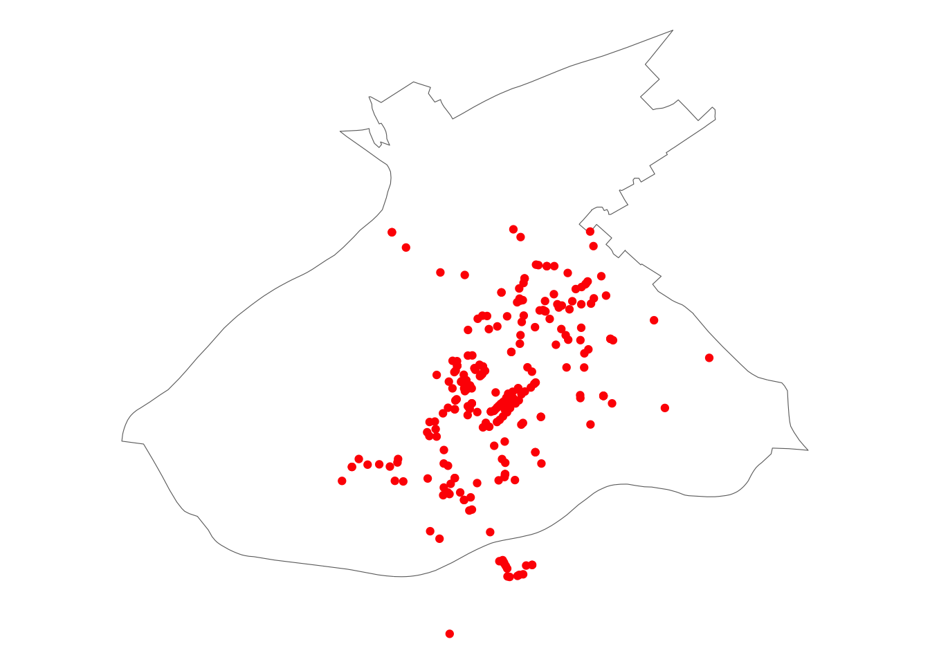

You can see more clearly now that there are some venues (in red) that fall outside of our desired boundary (of the city centre here). So what we expect that with the spatial operation we will exclude the venues that are outside our boundary, and include only those who are inside. We use st_intersects() to find which points fall within the polygon, and then we subset using this information.

# intersection
cc_intersects <- st_intersects(cc_WGS84, cc_spatial)
# subsetting
cc_intersects <- cc_spatial[unlist(cc_intersects),]

Have a look at this new cc_intersects object in your environment. How many observations does it have? Is this now fewer than the previous cc_spatial object? Why do you think this is? (hint: you’re removing everything that is outside the city centre polygon)

We can plot this too to have a look:

ggplot() + 
   # plot boundary with empty fill
  geom_sf(data = cc_WGS84, fill=NA) +
  # plot points in red
  geom_sf(data = cc_intersects, col = "red") + 
  # remove chart backgrounds
  theme_void()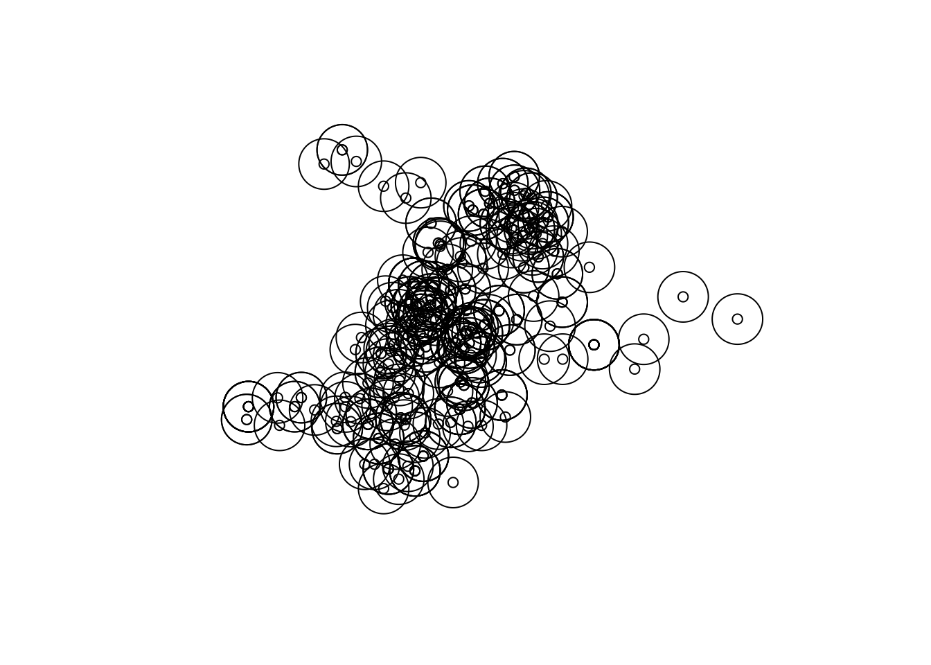

You can see now that any points that were outside the boundary are no longer in our dataset. COOL, we have successfully performed our first spatial operation, we managed to subset our points data set to include only those points which are inside the polgon for city centre. See how this was much easier, and more reliable than the hacky workaround using pattern matching? Yay!

4.8.4 Activity 6: Building buffers

Right, but what we want to do really to go back to our original question. We want to know about crime in and around out areas of interest, in this case our licensed premises. But how can we count this?

Well first we will need crime data. Let’s use the same data set from last week. I’m not going over the detail of how to read this in, if you forgot, go back to the notes from last week.

crimes <- read_csv("data/crimes_w_lsoa_codes_attached.csv")

## Rows: 32058 Columns: 12
## ── Column specification ────────────────────────────────
## Delimiter: ","
## chr (9): Crime.ID, Month, Reported.by, Falls.within, Location, Crime.type, L...
## dbl (2): Longitude, Latitude
## lgl (1): Context
## 
## ℹ Use `spec()` to retrieve the full column specification for this data.
## ℹ Specify the column types or set `show_col_types = FALSE` to quiet this message.

Notice that in this case the columns are spelled with upper case “L”. You should always familiarise yourself with your data set to make sure you are using the relevant column names. You can see just the column names using the names() function like so :

names(crimes)

##  [1] "Crime.ID"              "Month"                 "Reported.by"          
##  [4] "Falls.within"          "Longitude"             "Latitude"             
##  [7] "Location"              "Crime.type"            "Last.outcome.category"
## [10] "Context"               "lsoa21cd"              "lsoa21nm"

Arg so messy! Let’s use our handy helpful clean_names() function from the janitor package:

crimes <- crimes %>% clean_names()
names(crimes)

##  [1] "crime_id"              "month"                 "reported_by"          
##  [4] "falls_within"          "longitude"             "latitude"             
##  [7] "location"              "crime_type"            "last_outcome_category"
## [10] "context"               "lsoa21cd"              "lsoa21nm"

Or you can have a look at the first 6 lines of your dataframe with the head() function:

head(crimes)

## # A tibble: 6 × 12
##   crime_id month reported_by falls_within longitude latitude location crime_type
##   <chr>    <chr> <chr>       <chr>            <dbl>    <dbl> <chr>    <chr>     
## 1 <NA>     2019… Greater Ma… Greater Man…     -2.46     53.6 On or n… Anti-soci…
## 2 aa1cc4c… 2019… Greater Ma… Greater Man…     -2.44     53.6 On or n… Violence …
## 3 e513df6… 2019… Greater Ma… Greater Man…     -2.44     53.6 On or n… Violence …
## 4 6ed763d… 2019… Greater Ma… Greater Man…     -2.44     53.6 On or n… Violence …
## 5 780d55b… 2019… Greater Ma… Greater Man…     -2.45     53.6 On or n… Violence …
## 6 753fa25… 2019… Greater Ma… Greater Man…     -2.44     53.6 On or n… Violence …
## # ℹ 4 more variables: last_outcome_category <chr>, context <lgl>,
## #   lsoa21cd <chr>, lsoa21nm <chr>

Or you can view, with the View() function.

Now, we have our points that are crimes, right? Well… How do we connect them to our points that are licensed premises?

First things first, let’s make sure again that R is aware that this is a spatial set of points, and that the columns latitude and longitude are used to create a geometry.

crimes_spatial <- st_as_sf(crimes, coords = c("longitude", "latitude"), 
                 crs = 4326, agr = "constant")

Next, we should find a way to link each crime to the licenced premise which we might count it against.

One approach is to build a buffer around our licensed premises, and say that we will count all the crimes which fall within a specific radius of this licensed premise. What should this radius be? Well this is where your domain knowledge as criminologist comes in. How far away would you consdier a crime to still be related to this pub? 400 meters? 500 meters? 900 meters? 1 km? What do you think? This is again one of them it depends questions. Whatever buffer you choose you should justify, and make sure that you can defend when someone might ask about it, as the further your reach obviously the more crimes you will include, and these might alter your results.

So, let’s say we are interested in all crimes that occur within 400 meters of each licensed premise. We chose 400m here as this is the recommended distance for accessible bus stop guidance, so basically as far as people should walk to get to a bus stop (TfL, 2008). So in this case, we want to take our points, which represent the licensed premises, and build buffers of 400 meters around them.

You can do with the st_buffer() function:

prem_buffer <- st_buffer(cc_intersects, 1)

You should get a warning here. This message indicates that sf assumes a distance value is given in degrees. This is because we have lat/long data (WSG 48)

One quick fix to avoid this message, is to convert to BNG:

prem_BNG <- st_transform(cc_intersects, 27700)

Now we can try again, with meters

prem_buffer <- st_buffer(prem_BNG, 400)

Let’s see how that looks:

ggplot() + 
  geom_sf(data = prem_buffer, fill = "grey") + 
  geom_sf(data = prem_BNG) + 
  theme_void()

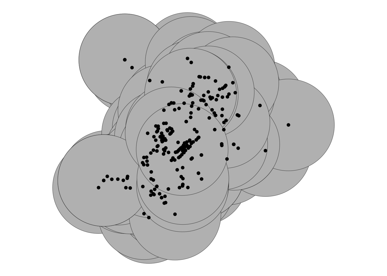
That should look nice and squiggly. But also it looks like there is quite a lot of overlap here. Should we maybe consider smaller buffers? Let’s look at 50 meter buffers:

prem_buffer_50 <- st_buffer(prem_BNG, 50)

ggplot() + 
  geom_sf(data = prem_buffer_50, fill = "grey") + 
  geom_sf(data = prem_BNG) + 
  theme_void()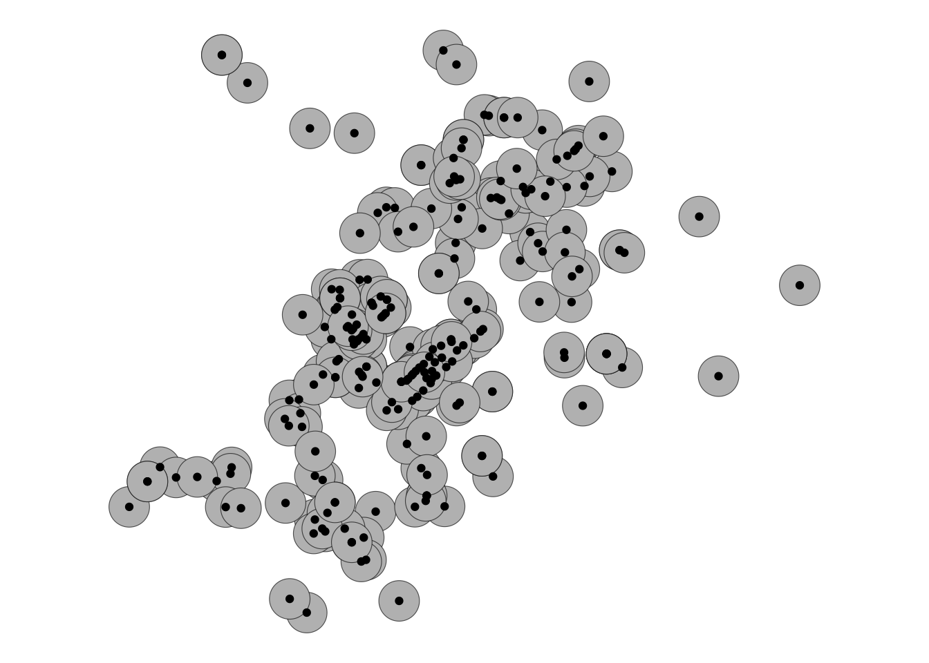

Still quite a bit of overlap, but this is possibly down to all the licensed premises being very densely close together in the city centre. And it seems like we can

Well now let’s have a look at our crimes. I think it might make sense (again using domain knowledge) to restrict the analysis to violent crime. So let’s do this:

violent_spatial <- crimes_spatial %>%
  filter(crime_type=="Violence and sexual offences")

Now, remember the CRS is WGS 48 here, so we will need to convert our buffer layer back to this:

buffer_WGS84 <- st_transform(prem_buffer_50, 4326)

Now, let’s get to our last spatial operation of the day, the famous points in polygon, to get to answering which licensed premises have the most violent crimes near them.

4.8.5 Activity 7: Counting Points in Polygon

When you have a polygon layer and a point layer - and want to know how many or which of the points fall within the bounds of each polygon, you can use this method of analysis. In computational geometry, the point-in-polygon (PIP) problem asks whether a given point in the plane lies inside, outside, or on the boundary of a polygon. As you can see, this is quite relevant to our problem, wanting to count how many crimes (points) fall within 100 meters of our licensed premises (our buffer polygons).

crimes_per_prem <- violent_spatial %>% 
  st_join(buffer_WGS84, ., left = FALSE) %>% 
  count(PREMISESNAME)

You now have a new dataframe, crimes_per_prem which has a column for the name of the premises, a column for the number of violent crimes that fall within the buffer, and a column for the geometry.

Take a moment to look at this table. Use the View() function. Which premises have the most violent crimes? Are you surprised?

Now as a final step, let’s plot this, going back to leaflet. We can shade by the number of crimes within the buffer, and include a little popup label with the name of the establishment:

pal <- colorBin("RdPu", domain = crimes_per_prem$n, bins = 5, pretty = TRUE)
leaflet(crimes_per_prem) %>% 
  addTiles() %>% 
  addPolygons(fillColor = ~pal(n), fillOpacity = 0.8,
              weight = 1, opacity = 1, color = "black",
              label = ~as.character(PREMISESNAME)) %>% 
  addLegend(pal = pal, values = ~n, opacity = 0.7, 
            title = 'Violent crimes', position = "bottomleft")

It’s not the neatest of maps, with all these overlap and it doesn’t allow us to see all the venues. Actually there is another issue here - we are double counting crimes. Here we asked the question: for each venue, how many crimes fall within a 50m buffer radius of it. This way we can build a sort of profile for the venue, considering whether it’s in a high crime area. This makes sense in this situation, because we don’t have more information than the locational proximity, we don’t know whether these offences are in any way connected to any venue.

If we did, and we wanted to assign each crime only once to only one venue, we could snap it to the nearest venue. Then we can count the number of crimes that had been snapped to each venue, and then use that to build our measure. The decision of which way to go comes back to your learnings around conceptualisation and operationalisation from your earlier data modules - it is so important that you clearly define what you mean when you consider your topic of study, and be clear about how you measure that and why that’s the best representation of your concept.

So before you go, let’s show you the approach where we snap each crime to the nearest venue, using st_nearest() function. First, we want to set a cut off, if the crime is more than some distance from our venues we don’t want to assign it. Here we can use our buffer spatial boundary. You will see, we will combine all our spatial operations in this one last exercise!

4.9 Activity 8: Combo!

First we want to take the buffers around all the venues, and unite them into one big boundary using st_union()

big_buffer <- st_union(prem_buffer_50)

# transform the crs of big_buffer to the crs of our violent crimes
big_buffer <- st_transform(big_buffer, 4326)

Then, we want to take only the violent crime incidents whic are within this big buffer using the st_intersects()

violence_in_buffer <- violent_spatial[unlist(st_intersects(big_buffer, violent_spatial)), ]

And now we can take these crimes and for each one, identify the nearest venue using st_nearest_feature() and then append the name of the nearest venue to this dataframe.

nearest_venues <- st_nearest_feature(violence_in_buffer, cc_intersects)
violence_in_buffer$nearest_prem <- cc_intersects$PREMISESNAME[nearest_venues]

We can now use this to build a frequency table of the number of crimes that are assigned to each venue:

crimes_per_prem_snapped <- violence_in_buffer %>%
  # st_set_geometry(NULL) %>%  # remove geometry for counting
  group_by(nearest_prem) %>%
  summarise(n = n())

And we can map these points again using leaflet:

# recreate the colour scheme we used with the previous map
pal <- colorBin("RdPu", domain = crimes_per_prem_snapped$n, bins = 5, pretty = TRUE)

# create a variable to adjust the size of the point by the value 
# so bigger circle for more crimes snapped
# but set a minimum value so smaller n venues still visible

crimes_per_prem_snapped <- crimes_per_prem_snapped %>%
  mutate(radius_m = pmax(n * 3, 30))  # 30 m minimum, scale factor = 5

leaflet(crimes_per_prem_snapped %>%  st_cast("POINT")) %>% 
  addTiles() %>% 
  addCircles(radius = crimes_per_prem_snapped$radius_m,
             fillColor = ~pal(n), fillOpacity = 0.8,
             weight = 1, opacity = 1, color = "black",
             label = ~as.character(nearest_prem)) %>% 
  addLegend(pal = pal, values = ~n, opacity = 0.7, 
            title = 'Violent crimes', position = "bottomleft")

## Warning in st_cast.MULTIPOINT(X[[i]], ...): point from first coordinate only
## Warning in st_cast.MULTIPOINT(X[[i]], ...): point from first coordinate only
## Warning in st_cast.MULTIPOINT(X[[i]], ...): point from first coordinate only
## Warning in st_cast.MULTIPOINT(X[[i]], ...): point from first coordinate only
## Warning in st_cast.MULTIPOINT(X[[i]], ...): point from first coordinate only

You can see here that the Morrisons on the corner of piccadilly gardens has exploded as our most crime ridden venue. Do have a chat about what you think this means with your neighbour, or with one of the teaching team. But consider that we just picked the closest venue to snap the point to, with no information how related that incident is to the particular venue. In this case, while there may be some chance that that Morrisons is just a bit rough, but also it might just be the closest proximate venue to Piccadilly Gardens, which is known to all of us familiar with Manchester…

4.10 Summary

In this week we explored the differences between attribute and spatial operations, and we made great use of the latter in practicing spatial manipulation of data. These spatial operations allow us to manipulate our data in a way that lets us study what is going on with crime at micro-places. We introduced the idea of different crime places. Make sure to refer to the readings about crime attractors vs. crime generators, as well as developments, for example about crime radiators and absorbers as well.

We covered how to subset points within an area, build buffers around geometries, count the number of points in a point layer that fall within each polygon in a polygon layer, and turn non-spatial information such as an address into something we can map using geocoding. These spatial operations are just some of many, but we chose to cover as they have the most frequent application in crime analysis.