Chapter 13 Spatial heterogeneity and regression
13.1 Introduction
One of the challenges of spatial data is that we may encounter exceptions to stationary processes. There may be, for example, parameter variability across the study area. When we have homogeneity everything is the same everywhere, in terms of our regression equation, the parameters are constant. But as we illustrated via an interaction term in the last chapter, that may not be the case. We can encounter situations where a particular input has a different effect in parts of our study area. In this chapter we explore this issue and a number of solutions that have been proposed to deal with it. It goes without saying that having extreme heterogeneity creates technical problems for estimation. If everything is different everywhere we may have to estimate more parameters that we have data for.
One way of dealing with this is by imposing some form of structure, for example partitioning data for the United States to fit a separate model for Southern and Northern counties. Unlike data partition, full spatial regimes also imply using different coefficients for each subset of the data but you fit everything in one go. This is essentially the same as running as many models as subsets you have. As Anselin (2007) highlights, this corrects for heterogeneity but does not explain it. We can then test whether this was necessary, using a Chow test comparing the simpler model with the one where we allow variability. Of course, we can also include spatial dependence in these models.
Another way of dealing with heterogeneity is by allowing continuous variation, rather than discrete (as when we subset the data), of the parameters. A popular method for doing this is geographically weighted regression (GWR). This is a case of a local regression where you try to estimate a different set of parameters for each location and these parameters are obtained from a subset of observation using kernel regression. In traditional local regression we select the subset in the attribute space (observations with similar attributes), in GWR the local subset is defined in a geographical sense using a kernel (remember how we used kernels for density estimation to define a set of “neighbours”). We are estimating regression equations based on nearby locations as specified by our kernel and this produces a different coefficient for each location. As with kernel density estimation you can distinguish between fixed bandwidth and adaptive bandwidth.
For this chapter we will need to load the following packages:
library(tidyr)
library(dplyr)
# Packages for handling spatial data and for geospatial carpentry
library(sf)
library(sp)
library(spdep)
# Packages for regression and spatial regression
library(spatialreg)
# Packages for mapping and visualisation
library(tmap)
library(ggplot2)
# Packages with spatial datasets
library(geodaData)
# For geographicaly weighted regression
library(spgwr)
13.2 Spatial regimes
13.2.1 Fitting the constrained and the unconstrained models
To illustrate this solution we will go back to the “ncovr” data we explored last week and use the same spatial weight matrix as in the previous chapter. If you have read the Baller et al. (2001) paper that we are in a way replicating here, you could see they decided that they needed to run separate models for the South and the North. Let´s explore this here.
data("ncovr")
# We coerce the sf object into a new sp object
ncovr_sp <- as(ncovr, "Spatial")
## old-style crs object detected; please recreate object with a recent sf::st_crs()
## old-style crs object detected; please recreate object with a recent sf::st_crs()# Then we create a list of neighbours using 10 nearest neighbours criteria
xy <- coordinates(ncovr_sp)
nb_k10 <- knn2nb(knearneigh(xy, k = 10))
rwm <- nb2mat(nb_k10, style='W')
rwm <- mat2listw(rwm, style='W')
# remove redundant objects
rm(list = c("ncovr_sp", "xy", "nb_k10"))We can start by running a model for the whole country to use as a baseline model:
fit1_70 <- lm(HR70 ~ RD70 + PS70 + MA70 + DV70 + UE70, data = ncovr)
summary(fit1_70)##
## Call:
## lm(formula = HR70 ~ RD70 + PS70 + MA70 + DV70 + UE70, data = ncovr)
##
## Residuals:
## Min 1Q Median 3Q Max
## -21.12 -3.14 -1.02 1.90 69.75
##
## Coefficients:
## Estimate Std. Error t value Pr(>|t|)
## (Intercept) 11.1376 0.7602 14.65 <2e-16 ***
## RD70 4.1541 0.1147 36.23 <2e-16 ***
## PS70 1.1449 0.1165 9.82 <2e-16 ***
## MA70 -0.2080 0.0233 -8.94 <2e-16 ***
## DV70 1.4066 0.1064 13.22 <2e-16 ***
## UE70 -0.4268 0.0497 -8.59 <2e-16 ***
## ---
## Signif. codes:
## 0 '***' 0.001 '**' 0.01 '*' 0.05 '.' 0.1 ' ' 1
##
## Residual standard error: 6.03 on 3079 degrees of freedom
## Multiple R-squared: 0.328, Adjusted R-squared: 0.327
## F-statistic: 301 on 5 and 3079 DF, p-value: <2e-16A simple visualisation of the residuals suggest the model may not be optimal for the entire study region:
ncovr$res_fit1 <- fit1_70$residuals
ggplot(ncovr, aes(x = res_fit1, colour = as.factor(SOUTH))) +
geom_density() +
xlab("Residuals") +
scale_color_brewer(palette = "Set1", name = "Region (1 = South)") +
theme_bw()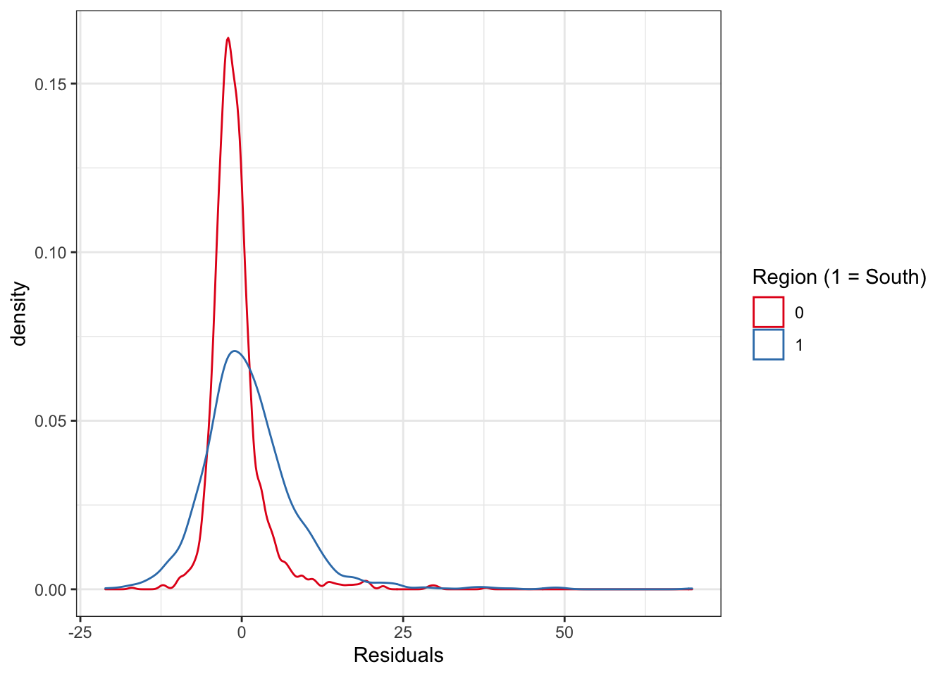
FIGURE 13.1: Distribution of residuals by study region (South v North)
To be able to fit these spatial regimes, that will allow for separate coefficients for counties in the North and those in the South, first we need to define a dummy for the Northern counties, and we create a vector of 1.
ncovr$NORTH <- recode(ncovr$SOUTH, `1` = 0, `0` = 1)
ncovr$ONE <- 1Having created these new columns we can fit a standard OLS model interacting the inputs with our dummies and setting the intercept to 0, so that each regime is allowed its own intercept:
fit2_70_sr <- lm(HR70 ~ 0 + (ONE + RD70 + PS70 + MA70 + DV70 + UE70):(SOUTH + NORTH),
data = ncovr)
summary(fit2_70_sr)##
## Call:
## lm(formula = HR70 ~ 0 + (ONE + RD70 + PS70 + MA70 + DV70 + UE70):(SOUTH +
## NORTH), data = ncovr)
##
## Residuals:
## Min 1Q Median 3Q Max
## -17.47 -2.79 -0.76 1.71 65.60
##
## Coefficients:
## Estimate Std. Error t value Pr(>|t|)
## ONE:SOUTH 15.0305 1.0714 14.03 < 2e-16 ***
## ONE:NORTH 6.6485 1.1308 5.88 4.6e-09 ***
## RD70:SOUTH 3.2364 0.1884 17.18 < 2e-16 ***
## RD70:NORTH 2.9523 0.2745 10.75 < 2e-16 ***
## PS70:SOUTH 0.9953 0.2114 4.71 2.6e-06 ***
## PS70:NORTH 0.8428 0.1402 6.01 2.0e-09 ***
## MA70:SOUTH -0.1656 0.0338 -4.90 1.0e-06 ***
## MA70:NORTH -0.1749 0.0325 -5.37 8.2e-08 ***
## DV70:SOUTH 0.6271 0.1750 3.58 0.00034 ***
## DV70:NORTH 1.4263 0.1313 10.86 < 2e-16 ***
## UE70:SOUTH -0.7916 0.0817 -9.69 < 2e-16 ***
## UE70:NORTH -0.0293 0.0631 -0.46 0.64265
## ---
## Signif. codes:
## 0 '***' 0.001 '**' 0.01 '*' 0.05 '.' 0.1 ' ' 1
##
## Residual standard error: 5.81 on 3073 degrees of freedom
## Multiple R-squared: 0.645, Adjusted R-squared: 0.644
## F-statistic: 465 on 12 and 3073 DF, p-value: <2e-16We can see a higher intercept for the South, reflecting the higher level of homicide in these counties. Aside from this, the two more notable differences are, on the one hand, the insignificant effect of unemployment in the North, and the higher impact of the divorce rate in the North.
13.2.2 Running the Chow test
The Chow Test is often used in econometrics to determine whether the independent variables have different impacts on different subgroups of the population. Anselin (2007) provides an implementation for this test, that extracts the residuals and the degrees of freedom from the constrained (the simpler oLS model) and the unconstrained models (the less parsimonious spatial regime), and then computes the test based on the F distribution.
chow.test <- function(rest,unrest)
{
er <- residuals(rest)
eu <- residuals(unrest)
er2 <- sum(er^2)
eu2 <- sum(eu^2)
k <- rest$rank
n2k <- rest$df.residual - k
c <- ((er2 - eu2)/k) / (eu2 / n2k)
pc <- pf(c,k,n2k,lower.tail=FALSE)
list(c,pc,k,n2k)
}With the function in our environment we can then run the test, which will yield the test statistic, the p value, and two degrees of freedom.
chow.test(fit1_70,fit2_70_sr)## [[1]]
## [1] 40.16
##
## [[2]]
## [1] 2.674e-47
##
## [[3]]
## [1] 6
##
## [[4]]
## [1] 3073How we interpret this test? When the Chow test is significant, as here, this provides evidence of spatial heterogeneity and in favour of fitting a spatial regime model, allowing for non-constant coefficients across the discrete subsets of data that we have specified.
13.2.3 Spatial dependence with spatial heterogeneity
So far we have only adjusted for a form of spatial heterogeneity in our model, but we may still have to deal with spatial dependence. Here what we covered in the previous chapter, still applies. We can run the various specification tests and then select a model that adjust for spatial dependence.
summary(lm.LMtests(fit2_70_sr, rwm, test = c("LMerr","LMlag","RLMerr","RLMlag")))## Lagrange multiplier diagnostics for spatial
## dependence
## data:
## model: lm(formula = HR70 ~ 0 + (ONE + RD70 +
## PS70 + MA70 + DV70 + UE70):(SOUTH + NORTH), data
## = ncovr)
## weights: rwm
##
## statistic parameter p.value
## LMerr 227.20 1 < 2e-16 ***
## LMlag 252.00 1 < 2e-16 ***
## RLMerr 5.25 1 0.022 *
## RLMlag 30.05 1 4.2e-08 ***
## ---
## Signif. codes:
## 0 '***' 0.001 '**' 0.01 '*' 0.05 '.' 0.1 ' ' 1The Lagrange multiplier tests, according to Anselin suggestions for how to interpret these, point to a spatial lag model (since RLMlag is several orders more significant than the error alternative).
We could then fit this model using sp
fit3_70_sr_sar <- lagsarlm(HR70 ~ 0 +
(ONE + RD70 + PS70 + MA70 + DV70 + UE70):(SOUTH + NORTH),
data = ncovr, rwm)
summary(fit3_70_sr_sar)##
## Call:
## lagsarlm(formula = HR70 ~ 0 + (ONE + RD70 + PS70 + MA70 + DV70 +
## UE70):(SOUTH + NORTH), data = ncovr, listw = rwm)
##
## Residuals:
## Min 1Q Median 3Q Max
## -17.15273 -2.66726 -0.67209 1.49219 65.86918
##
## Type: lag
## Coefficients: (asymptotic standard errors)
## Estimate Std. Error z value Pr(>|z|)
## ONE:SOUTH 8.391260 1.103507 7.6042 2.864e-14
## ONE:NORTH 4.903963 1.091437 4.4931 7.019e-06
## RD70:SOUTH 2.355243 0.191445 12.3025 < 2.2e-16
## RD70:NORTH 2.669956 0.266521 10.0178 < 2.2e-16
## PS70:SOUTH 0.653640 0.203791 3.2074 0.0013394
## PS70:NORTH 0.778913 0.135054 5.7674 8.050e-09
## MA70:SOUTH -0.100568 0.032699 -3.0756 0.0021009
## MA70:NORTH -0.138235 0.031328 -4.4126 1.022e-05
## DV70:SOUTH 0.636867 0.168184 3.7867 0.0001527
## DV70:NORTH 1.157985 0.128559 9.0074 < 2.2e-16
## UE70:SOUTH -0.522353 0.079210 -6.5945 4.267e-11
## UE70:NORTH -0.039129 0.060706 -0.6446 0.5192148
##
## Rho: 0.3957, LR test value: 181.8, p-value: < 2.22e-16
## Asymptotic standard error: 0.02846
## z-value: 13.9, p-value: < 2.22e-16
## Wald statistic: 193.3, p-value: < 2.22e-16
##
## Log likelihood: -9710 for lag model
## ML residual variance (sigma squared): 31.21, (sigma: 5.587)
## Number of observations: 3085
## Number of parameters estimated: 14
## AIC: 19448, (AIC for lm: 19628)
## LM test for residual autocorrelation
## test value: 0.7147, p-value: 0.39789We see that the AIC is better than for the non-spatial model and that there is no more residual autocorrelation. We could explore other specifications (ie spatial Durbin model) and the same caveats about interpreting coefficients in a spatial lag model we raised in the previous chapter would apply here. If the Lagrange multiplier tests had suggested a spatial error model, we could also have fitted the model in the way we have also already covered simply adjusting the regression formula as in this section.
We can now also run a Chow test, only in this case, we need to adjust the previous one to account for spatial dependence. Anselin (2007) also provides for an implementation of this test in R with the following ad-hoc function:
spatialchow.test <- function(rest,unrest)
{
lrest <- rest$LL
lunrest <- unrest$LL
k <- rest$parameters - 2
spchow <- - 2.0 * (lrest - lunrest)
pchow <- pchisq(spchow,k,lower.tail=FALSE)
list(spchow,pchow,k)
}This function will test a spatial lag model for the whole country as a whole with the spatial lag model with our data partitions. So first we need to estimate the appropriate lag model to be our constrained model:
fit4_70_sar <- lagsarlm(HR70 ~ RD70 + PS70 + MA70 + DV70 + UE70, data = ncovr,
rwm)Which we can then use in the newly created function:
spatialchow.test(fit4_70_sar, fit3_70_sr_sar)## [[1]]
## [,1]
## [1,] 58.59
##
## [[2]]
## [,1]
## [1,] 8.712e-11
##
## [[3]]
## [1] 6The test is again highly significant providing evidence for the spatial lag model with the spatial regimes.
13.3 Geographically Weighted Regression
The basic idea behind Geographically Weighted Regression (GWR) is to explore how the relationship between a dependent variable (\(Y\)) and one or more independent variables (the \(X\)s) might vary geographically. Instead of assuming that a single model can be fitted to the entire study region, it looks for geographical differences in the relationship. This is achieved by fitting a regression equation to every feature in the dataset. We construct these separate equations by incorporating the dependent and explanatory variables of the features falling within the neighborhood of each target feature.
Geographically Weighted Regression can be used for a variety of applications, including the following:
- Is the relationship between homicide rate and resource deprivation consistent across the study area?
- What are the key variables that explain high homicide rates?
- Where are the counties in which we see high homicide rates? What characteristics seem to be associated with these? Where is each characteristic most important?
- Are the factors influencing higher homicide rates consistent across the study area?
GWR provides three types of regression models: Continuous, Binary, and Count. These types of regression are known in statistical literature as Gaussian, Logistic, and Poisson, respectively. The Model Type for your analysis should be chosen based on the level of measurement of the Dependent Variable \(Y\).
So to illustrate, let us first build our linear model once again, regressing homicide rate in the 1970s for each county against resource deprivation (RD70), population structure (PS70), median age (MA70), divorce rate (DV70), and unemployment rate (UE70).
# make linear model
model <- lm(HR70 ~ RD70 + PS70 + MA70 + DV70 + UE70, data = ncovr)
summary(model)##
## Call:
## lm(formula = HR70 ~ RD70 + PS70 + MA70 + DV70 + UE70, data = ncovr)
##
## Residuals:
## Min 1Q Median 3Q Max
## -21.12 -3.14 -1.02 1.90 69.75
##
## Coefficients:
## Estimate Std. Error t value Pr(>|t|)
## (Intercept) 11.1376 0.7602 14.65 <2e-16 ***
## RD70 4.1541 0.1147 36.23 <2e-16 ***
## PS70 1.1449 0.1165 9.82 <2e-16 ***
## MA70 -0.2080 0.0233 -8.94 <2e-16 ***
## DV70 1.4066 0.1064 13.22 <2e-16 ***
## UE70 -0.4268 0.0497 -8.59 <2e-16 ***
## ---
## Signif. codes:
## 0 '***' 0.001 '**' 0.01 '*' 0.05 '.' 0.1 ' ' 1
##
## Residual standard error: 6.03 on 3079 degrees of freedom
## Multiple R-squared: 0.328, Adjusted R-squared: 0.327
## F-statistic: 301 on 5 and 3079 DF, p-value: <2e-16And now, to get an idea of how our model might perform differently in different area, we can map the residuals across each county:
# map residuals
ncovr$resids <- residuals(model)
qtm(ncovr, fill = "resids")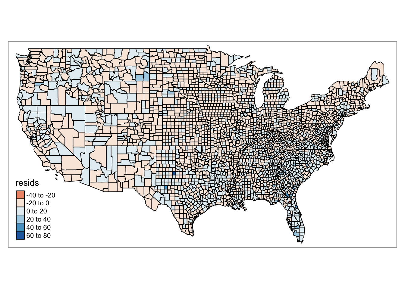
FIGURE 13.2: Map of model residuals
If we see that there is a geographic pattern in the residuals, it is possible that an unobserved variable may be influencing the dependent variable, and there might be some sort of spatial variation in our model’s performance. This is what GWR allows us to explore, whether the relationship between our variables is stable over space.
13.3.1 Calculate kernel bandwidth
The big assumption on which the GWR model is based is the kernel bandwitdh. As mentioned earlier, in order to calculate local coefficients for our study regions, GWR takes into account the data points within our specified bandwith, weighting them appropriately. The bendwidth we choose will determine our results. If we choose something too large, we might mask variation, and get resuls similar to the global results. If we choose something too small, we might get spikes, and lots of small scale variation, but also possibly large standard errors and unreliable estimates. Therefore, the process of choosing an appropriate bandwidth is paramount to GWR.
It is possible that we choose bandwidth manually, based on some prior knowledge, or theoretically based argument. However, if we do not have such ideas to start, we can use data-driven processes to inform our selection. The most frequently used approach is to use cross validation. Other approaches include Akaike Information Criteria, and maximum likelihood.
Here we use gwr.sel() which uses cross validation method for selecting optimal method for GWR. The function finds a bandwidth for a given geographically weighted regression by optimizing a selected function. For cross-validation, this scores the root mean square prediction error for the geographically weighted regressions, choosing the bandwidth minimizing this quantity.
With adapt function you can choose whether you want the bandwidth to adapt (i.e. find the proportion between 0 and 1 of observations to include in weighting scheme (k-nearest neighbours)) or whether you want to find a global bandwidth. A global bandwidth might make sense where the areas of interest are of equal size, and equally spaced, however if we have variation, for example like in the case of the counties of the United States, it makes sense to adjust the bandwidth for each observation. Here we set to adapt.
Another important consideration is the function for the geographical weighting. We mentioned this above. In the gwr.sel() function you can set this with the gweight= parameter. By default, this is set to a Gaussian function. We will keep it that way here.
With an sf object (whcih our data are in), one of the parameters required is a coordinate point for each one of our observations. In this case, what we can do is grab the centroid of each one of our polygons. To do this, we can use the st_coordinates() function:
ncovr <- ncovr %>%
mutate(cent_coords = st_coordinates(st_centroid(.)))Now that we have our centroids, we can calculate our optimal bandwith, and save this into an object called gwr_bandwidth.
gwr_bandwidth <- gwr.sel(HR70 ~ RD70 + PS70 + MA70 + DV70 + UE70,
data = ncovr,
coords = ncovr$cent_coords,
adapt = T)## Adaptive q: 0.382 CV score: 109039
## Adaptive q: 0.618 CV score: 110549
## Adaptive q: 0.2361 CV score: 107560
## Adaptive q: 0.1459 CV score: 105925
## Adaptive q: 0.09017 CV score: 104176
## Adaptive q: 0.05573 CV score: 102283
## Adaptive q: 0.03444 CV score: 100199
## Adaptive q: 0.02129 CV score: 98707
## Adaptive q: 0.01316 CV score: 98388
## Adaptive q: 0.01161 CV score: 98447
## Adaptive q: 0.01475 CV score: 98373
## Adaptive q: 0.0145 CV score: 98390
## Adaptive q: 0.01725 CV score: 98566
## Adaptive q: 0.01571 CV score: 98411
## Adaptive q: 0.01512 CV score: 98356
## Adaptive q: 0.01534 CV score: 98364
## Adaptive q: 0.01508 CV score: 98358
## Adaptive q: 0.01517 CV score: 98354
## Adaptive q: 0.01524 CV score: 98351
## Adaptive q: 0.01528 CV score: 98356
## Adaptive q: 0.01524 CV score: 98351So we now have our bandwidth. It is:
gwr_bandwidth## [1] 0.01524As our data are in WGS84 this value is in degrees.
13.3.2 Building the geographically weighted model
Now we can build our model. The gwr() function implements the basic geographically weighted regression approach to exploring spatial non-stationarity for given bandwidth and chosen weighting scheme. We specify the formula and our data soucre, as with the linear and spatial regressions, and the coords of the centroids, as we did in the bandwidth calculation above, but now we also specify our bandwith, which we created earlier, but we do this with the adapt= parameter. This is because, by default, the function takes a global bandwidth with the bandwidth= parameter, and we have created an adaptive bandwidth, so we shall use this adapt= parameter to include our GWRbandwidth object. We also set the hatmatrix = parameter to TRUE, to return the hatmatrix as a component of the result, and the se.fit= parameter to TRUE to return local coefficient standard errors - as we set hatmatrix to TRUE, two effective degrees of freedom sigmas will be used to generate alternative coefficient standard errors.
gwr_model = gwr(HR70 ~ RD70 + PS70 + MA70 + DV70 + UE70, data = ncovr,
coords = ncovr$cent_coords,
adapt=gwr_bandwidth,
hatmatrix=TRUE,
se.fit=TRUE)
gwr_model## Call:
## gwr(formula = HR70 ~ RD70 + PS70 + MA70 + DV70 + UE70, data = ncovr,
## coords = ncovr$cent_coords, adapt = gwr_bandwidth, hatmatrix = TRUE,
## se.fit = TRUE)
## Kernel function: gwr.Gauss
## Adaptive quantile: 0.01524 (about 47 of 3085 data points)
## Summary of GWR coefficient estimates at data points:
## Min. 1st Qu. Median 3rd Qu. Max.
## X.Intercept. -4.2897 4.4361 7.4395 12.3212 30.1335
## RD70 -0.3625 2.0168 2.8788 3.8206 6.6405
## PS70 -4.0630 0.2914 1.0987 1.9019 3.4998
## MA70 -0.6831 -0.2072 -0.1028 -0.0186 0.2971
## DV70 -0.7513 0.5368 0.9652 1.4351 3.1027
## UE70 -1.4895 -0.4286 -0.1787 -0.0220 1.8486
## Global
## X.Intercept. 11.14
## RD70 4.15
## PS70 1.14
## MA70 -0.21
## DV70 1.41
## UE70 -0.43
## Number of data points: 3085
## Effective number of parameters (residual: 2traceS - traceS'S): 244
## Effective degrees of freedom (residual: 2traceS - traceS'S): 2841
## Sigma (residual: 2traceS - traceS'S): 5.405
## Effective number of parameters (model: traceS): 171.2
## Effective degrees of freedom (model: traceS): 2914
## Sigma (model: traceS): 5.337
## Sigma (ML): 5.186
## AICc (GWR p. 61, eq 2.33; p. 96, eq. 4.21): 19276
## AIC (GWR p. 96, eq. 4.22): 19082
## Residual sum of squares: 82986
## Quasi-global R2: 0.5022This output tells us the 5-number summary for the coefficients (\(Y\)) for each predictor variable \(X\). We can see for all predictor variables, some counties have negative values, while other counties have positive values. Evidently there is some variation locally in the relationships between these independent variables and our dependent variable.
For this to be informative however, we should map this variation - this is where we can gain insight into how the relationships may change over our study area. In our gwr_model object we have a Spatial Data Frame. This is a SpatialPointsDataFrame or SpatialPolygonsDataFrame object which contains fit.points, weights, GWR coefficient estimates, R-squared, and coefficient standard errors in its “data” slot. Let’s extract this into another object called gwr_results:
gwr_results <- as.data.frame(gwr_model$SDF)To map this, we can join these results back to our original data frame.
gwr_results <- cbind(ncovr, gwr_results)Now we can begin to map our results. First, let’s see how well the model performs across the different counties of the United States. To do this, we can map the localR2 value which contains the local \(R^2\) value for each observation.
qtm(gwr_results, fill = "localR2" )## old-style crs object detected; please recreate object with a recent sf::st_crs()
## old-style crs object detected; please recreate object with a recent sf::st_crs()
## old-style crs object detected; please recreate object with a recent sf::st_crs()
## old-style crs object detected; please recreate object with a recent sf::st_crs()
## old-style crs object detected; please recreate object with a recent sf::st_crs()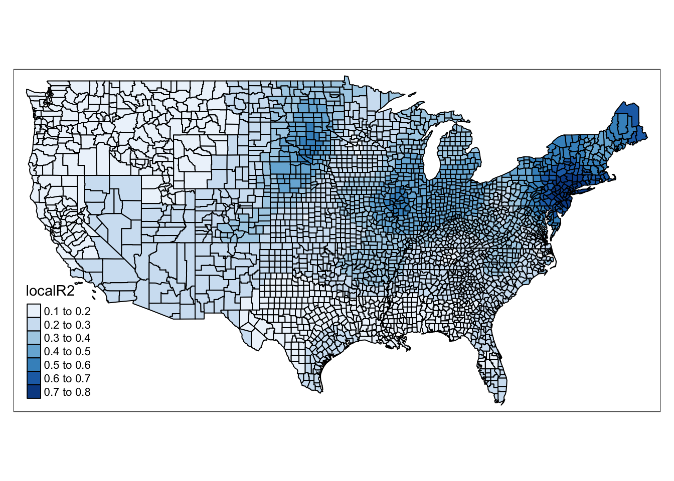
FIGURE 13.3: Map of local R-square value for each county
We can see some really neat spatial patterns in how well our model performs in various regions of the United States. Our model performs really well in the North East for example, but not so well in the South.
We can also map the coefficients for specific variables. Let’s say we’re interested in how the relationship between Resource deprivation (RD70) and homicide rate.
NOTE: In our
gwr_resultsdata frame we have a varaible calledRD70, this contains the observed resource deprivation value for the county. We then haveRD70.1this is the coefficient value for each county. In the results contained in the SDF element of our model (gwr_model$SDF) it was namedRD70but when we joined the two object, the.1was appended to allow us to differentiate between the two.
qtm(gwr_results, fill = "RD70.1" )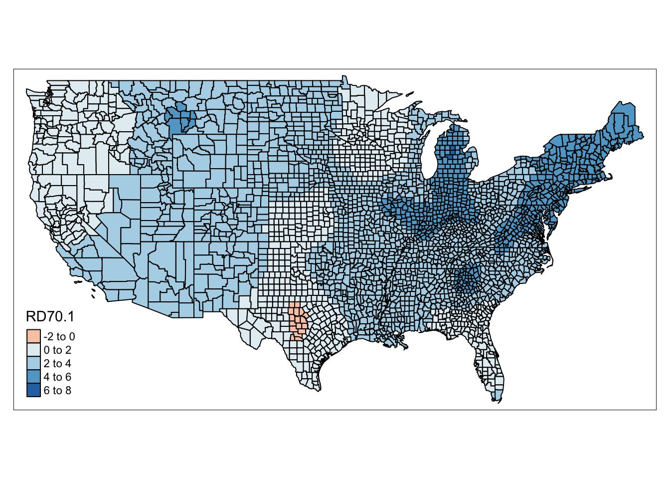
FIGURE 13.4: Map of coefficient for resource deprivation value for each county
We can see in this map again some regional patterns in the coefficient of Resource deprivation. There are even counties, in Texas, and in Florida, where the direction of this relationship flips, that is we have negative coefficients - so resource deprivation is associated with lower homicide rates in these counties.
This may be interesting and raise questions, however, it is important to consider not only the coefficients, but also the standard errors associated with them, so we can get some ideas behind the reliability of these estimates. So let us have a look by mapping the standard errors for these coefficients, which are contained in the RD70_se variable.
qtm(gwr_results, fill = "RD70_se" )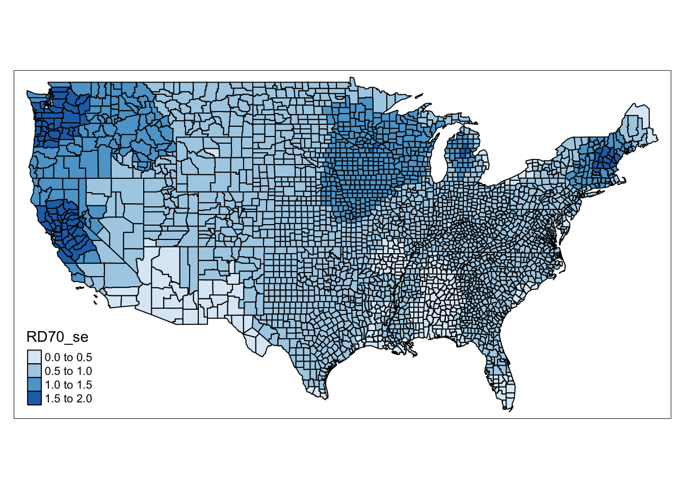
FIGURE 13.5: Map of standard error for resource deprivation value for each county
Higher standard errors mean that our estimates may be less reliable. So it is important to keep in mind both maps, the one with the coefficients, and the one showing the standard errors, when drawing conclusions from our GWR results.
13.3.3 Using GWR
Overall, GWR is a good exploratory tool which can help illustrate how a particular model might apply differently in different regions of your study area, or how relationships between variables may vary spatially. This technique can be extended, for example to count models, or logit models, but (following the lead of Luc Anselin) we stop here, and pause to highlight some issues. Specifically, our results are very sensitive to our choice of bandwidth. The results we achieve with this approach might not show up when we use other bandwiths. Additionally, GWR does not really explain anything. What we do, is demonstrate that the relationship between our variables is not stable over space. But we cannot with this technique explain why it is not stable over space.
Nevertheless it is a great technique to identify spatial variation, which, unlike spatial regimes, does not rely on our a-priory segmentation of our study region, but instead allows for the variation to emerge from the data themselves.
13.4 Summary and further reading
This chapter has tackled some of the issues of spatial heterogeneity in regression results. When applying regression in a spatial context, it is possible to encounter situations where we might observe a different effect on our variables in different parts of our study area. SPecifically, we covered two approaches to exploring this. The first one was to impose some a-priori segmentation to our data, based on contextual knowledge and possible patterns in our regression results. We illustrated this by imposing spatial regimes in our NCOVR data set, splitting into separate North and South USA, as was done by the original authors of the paper Baller et al. (2001). The second approach was to explore how the coefficients may vary across our study space by applying Geographically Weighted Regression to our study area. We provided a high-level overview of this process and recommended it as an illustrative, exploratory technique to raise questions about possible spatial heterogeneity in the processes we are trying to model in our study region.
To delve into greater detail on the topic of spatial heterogeneity, Chapters 8 and 9 in Anselin (2007) discuss specification of spatial heterogeneity. This is particularly helpful as an introduction to the issues and solutions we have discussed in this chapter. For more details and applications of Geographically Weighted Regression, we recommend Fotheringham, Brunsdon, and Charlton (2003). For applications and an illustration of the importance to consider spatial variation within the context of criminology and crime analysis, read Cahill and Mulligan (2007) and Andresen and Ha (2020) as good examples.
And for those wishing to explore additional ways to model spatial interactions, such as CAR and Bayesian models, we suggest to read Banerjee, Carlin, and Gelfand (2014) as well as Chapters 9 and 10 in Bivand, Pebesma, and Gómez-Rubio (2013).