Chapter 8 Spatial point patterns of crime events
8.1 Mapping crime intensity with isarithmic maps
A key piece of information we explore in environmental criminology is the “exact” location of crimes, typically in the form of street address in which a crime is recorded as having occurred. A key goal of the analysis of this type of mapped point data is to detect patterns, in particular to detect areas where crime locations appear as clustered and reflecting an increased likelihood of occurrence.
In Chapter 1, we generated some maps with point locations representing crimes in Greater Manchester (UK) and we saw how the large volume of events made it difficult to discern any spatial pattern. In previous chapters we saw how we could deal with this via aggregation of the point data to enumeration areas such census tracts or by virtue of binning. In this chapter we will introduce techniques that are used as an alternative visualisations for point patterns and that are based on the mathematics of density estimation. They are used to produce isarithmic maps, these are the kind of maps you often see in the weather reports displaying temperature. What we are doing is creating an interpolated surface from discrete data points. Or in simpler terms we are “effectively inventing data values for the areas on the map for which you don’t have data or sample points” (Field 2015).
Before we get to the detail of how we produce these maps we will briefly and very generally introduce the field of spatial point pattern analysis. The analysis of discrete locations are a subfield of spatial statistics. In this chapter we will introduce an R package called spatstat, that was developed for spatial point pattern analysis and modelling. It was written by Adrian Baddeley and Rolf Turner. There is a webpage and a book (Baddeley, Rubak, and Turner 2015) dedicated to this package. In our book we are only going to provide you with an introductory practical entry into this field of techniques. If this package is not installed in your machine, make sure you install it before we carry on. In this chapter we will also be using the package crimedata developed by our colleague Matt Ashby, which we introduced in the previous Chapter (Ashby 2018).
# Packages for reading data and data carpentry
library(readr)
library(dplyr)

# Packages for handling spatial data and for geospatial carpentry
library(sf)
library(maptools)
library(raster) # used for data represented in a raster model

# Specific packages for spatial point pattern analysis
library(spatstat)

# Libraries for spatial visualisation
library(tmap)
library(ggplot2)
library(leaflet)

# Libraries with relevant data for the chapter
library(crimedata)
8.2 Burglaries in NYC
Like in Chapter 6, our data come from the Crime Open Database (CODE), a service that makes it convenient to use crime data from multiple US cities in research on crime. All the data in CODE are available to use for free as long as you acknowledge the source of the data. The package crimedata was developed by Dr. Ashby to make it easier to read into R the data from this service. In the last chapter we provided the data in a csv format, but here we will actually make use of the package to show you how you might acquire such data yourself.
The key function in crimedata is get_crime_data(). We will be using the crime data from New York City police and for 2010, and we want the data to be in sf format. We will also filter the data to only include residential burglaries in Brooklyn.
# Large dataset, so it will take a while
nyc_burg <- get_crime_data(
  cities = "New York", #specifies the city for which you want the data
  years = 2010,        #reads the appropriate year of data
  type = "extended",   #select extended (a fuller set of fields)
  output = "sf") %>%        #return a sf object (vs tibble)
filter(offense_type == "residential burglary/breaking & entering" &
           nyc_boro_nm == "MANHATTAN")
Additionally we will need a geometry of borough boundaries. We have downloaded this from the NYC open data portal, and is supplied with the data included with this book. The file is manhattan.geojson.
manhattan <- st_read("data/manhattan.geojson") %>%
  filter(BoroName == "Manhattan") # select only Manhattan
Now we have all our data, let’s plot to see how they look.
ggplot() +
  geom_sf(data = manhattan) + # boundary data
  geom_sf(data = nyc_burg, size = 0.5) +  # crime locations as points
  theme_void()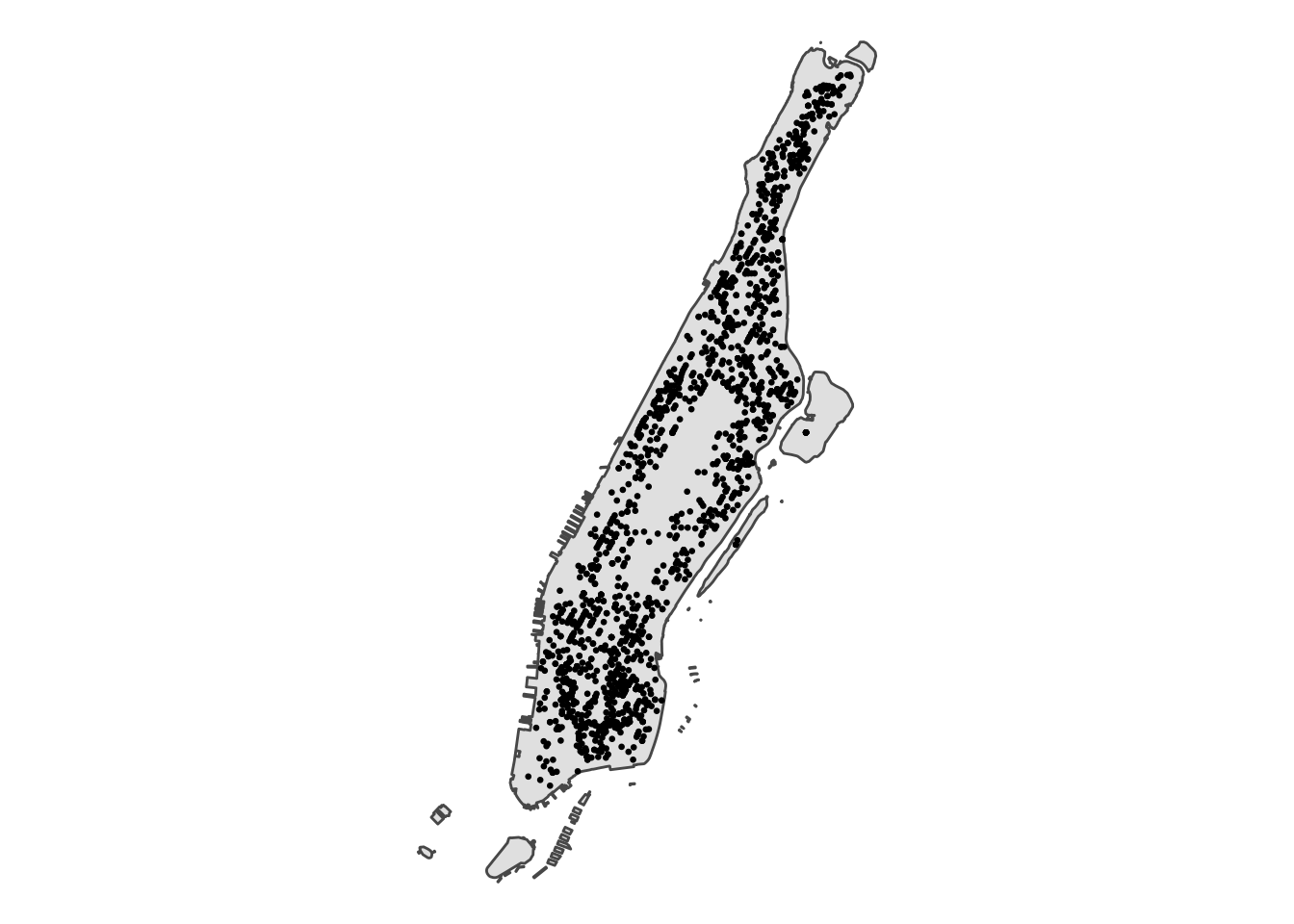
FIGURE 8.1: Plot Manhattan borough and crime locations as points
In the point pattern analysis literature each point is often referred to as an event and these events can have marks, attributes or characteristics that are also encoded in the data. In our spatial object one of these marks is the type of crime (although in this case it is of little interest since we have filtered on it). Others in this object include the date and time, the location category, victim sex and race, etc.
8.3 Using the spatstat package
The R package spatstat was created for spatial statistics with a strong focus on analysing spatial point patterns. It is the result of 15 years’ development by leading researchers in spatial statistics. We highly recommend the book “Spatial Point Patterns: Methodology and Applications with R” to give a comprehensive overview of this package (Baddeley, Rubak, and Turner 2015).
When working within the spatstat environment, we will be working with planar point pattern objects. This means that the first thing we need to do is to transform our sf object into a ppp (planar point pattern) object. This is how spatstat likes to store its point patterns. The components of a ppp object include the coordinates of the points and the observation window (defining the study area).
It is important to realise that a point pattern is defined as a series of events in a given area, or window, of observation. Therefore we need to precisely define this window. In spatstat the function owin() is used to set the observation window. However, the standard function takes the coordinates of a rectangle or of a polygon from a matrix, and therefore it may be a bit tricky to use with a sf object. Luckily the package maptools provides a way to transform a SpatialPolygons into an object of class owin, using the function as.owin(). Here are the steps.
First, we transform the CRS of our Manhattan polygon into projected coordinates as opposed to the original geographic coordinates (WGS84), since only projected coordinates may be converted to spatstat class objects. As we saw in chapter 2, measuring distance in meters is a bit easier, so since with points a good deal of the analysis we subject them to involve measuring their distance from each other, moving to a projected system makes sense. For NYC the recommended projection is the New York State Plane Long Island Zone (EPSG 2263), that provides a high degree of accuracy and balances size and shape well. This projection, however, uses US feet (which will be deprecated in 2022), so instead we are going to use EPSG 32118, as an alternative that uses meters as unit of measurement. So first, transform our object using st_transform():
manhattan <- st_transform(manhattan, 32118)Then we use the as.owin() function to define the window based on our manhattan object.
window <- as.owin(st_geometry(manhattan))We can plot this window to see if it looks similar in shape to our polygon of Manhattan.
plot(window) # owin similar to polygon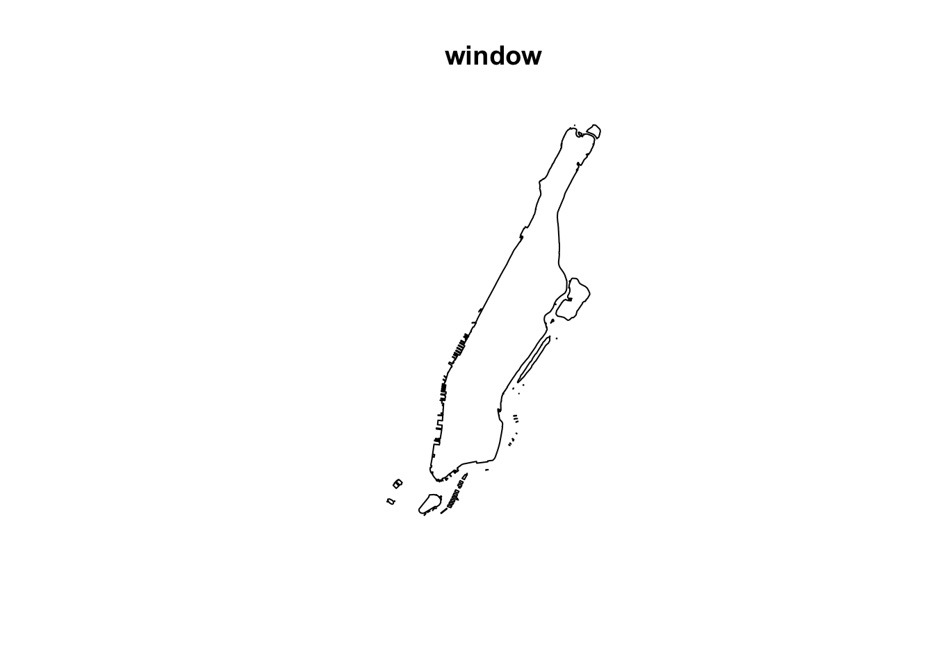
FIGURE 8.2: Plot window based on Manhattan polygon
We can see this worked and created an owin object.
class(window)## [1] "owin"window## window: polygonal boundary
## enclosing rectangle: [295965, 307869] x [57329, 79111]
## unitsYou can see it prints the units of measurement. But it does not identify them:
unitname(window)## unit / unitsAs noted above, EPGS:32118 uses meters. So we can pass this information to our owin object:
unitname(window) <- "Meter"Now that we have created the window as an owin object let’s get the points. In the first place we need to reproject to the same projected coordinate systems we have for our boundary data using the familiar st_transform() function from sf. Then we will extract the coordinates from our sf point data into a matrix using unlist() from base R, so that the functions from statspat can read the coordinates. If you remember sf objects have a column called geometry that stores these coordinates as a list. By unlisting we are flattening this list, taking the elements out of the list.
# first transform to projected CRS too to match our window
nyc_burg <- st_transform(nyc_burg, 32118)

# create matrix of coordinates
sf_nyc_burg_coords <- matrix(unlist(nyc_burg$geometry), ncol = 2, byrow = T)
Then we use the ppp() function from the spatstat package to create the object using the information from our matrix and the window that we created. The check argument is a logical that specifies whether we want to check that all points fall within the window of observation. It is recommended to set it to TRUE, unless you are absolutely sure that this is unnecessary.
bur_ppp <- ppp(x = sf_nyc_burg_coords[,1], y = sf_nyc_burg_coords[,2],
                   window = window, check = T)
## Warning: data contain duplicated pointsNotice the warning message about duplicated points? In spatial point pattern analysis an issue of significance is the presence of duplicates. The statistical methodology used for spatial point pattern processes is based largely on the assumption that processes are simple, that is, that the points cannot be coincident. That assumption may be unreasonable in many contexts (for example, the literature on repeat victimisation indeed suggests that we should expect the same addressess to be at a higher risk of being hit again). Even so, the point (no pun intended) is that “when the data has coincidence points, some statistical procedures will be severely affected. So it is always strongly advisable to check for duplicate points and to decide on a strategy for dealing with them if they are present” (Baddeley, Rubak, and Turner 2015: p. 60).
So how to perform this check? When creating the object above, we have already been warned this is an issue. But more generally we can check the duplication in a ppp object with the following syntax: it will return a logical indicating whether we have any duplication:
any(duplicated.ppp(bur_ppp))## [1] TRUETo count the number of coincidence points we use the multiplicity() function from the spatstat package. This will return a vector of integers, with one entry for each observation in our dataset, giving the number of points that are identical to the point in question (including itself).
multiplicity(bur_ppp)If you suspect many duplicates, it may be better start asking how many there are. For this you can use:
sum(multiplicity(bur_ppp) > 1)## [1] 915That’s quite something! 915 points out of 1727 burglaries share the same coordinates. And we can plot this vector if we want to see the distribution of duplicates:
hist(multiplicity(bur_ppp))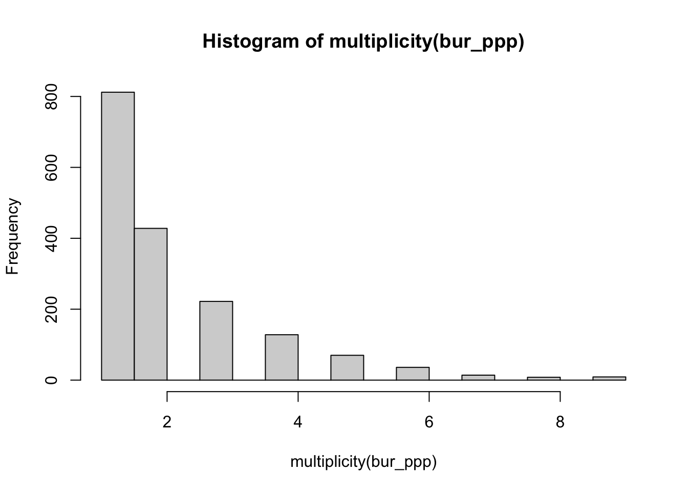
FIGURE 8.3: Histogram of incidents in overlapping coordinates (multiplicity)
In the case of crime, as we have hinted some of this may be linked to the nature of crime itself. Hint: repeat victimisation. It is estimated that between 7 and 33 % of all burglaries in several western and developed countries are repeat offenses (Chainey and Alves-da-Silva 2016). Our 52% is quite high by those standards. In this particular situation, it likely is the result of geomasking (the introduction of small inaccuracies into their geocoded location) due to privacy reasons. Most police data stored in open data portals do not include the exact address of crime events. In the case of US police data, as noted by the documentation of CODE, relies on addresses geocoded to the nearest hundred block. So say “370 Gorse Avenue” could be rounded down and geooded to “300 Gorse Avenue”. The same would happen to “307 Gorse Avenue”, in the public release version of the data it would feature as “300 Gorse Avenue”. In the UK there exist a pre-determined list of points so that each crime event gets “snapped” to its nearest one. So, the coordinates provided in the open data are not the exact locations of crimes. This process is likely inflating the amount of duplication we may observe, because each snap point or hundred block address might have many crimes near it, resulting in those crimes being geo-coded to the same exact location. So keep it in mind when analysing and working with this kind of data set that it may not be the same as working with the real locations. (If you are interested in the effects of this read the paper Tompson et al. (2015)).
What to do about duplicates in spatial point pattern analysis is not always clear. You could simply delete the duplicates, but of course that may ignore issues such as repeat victimisation. You could also use jittering, which will add a small perturbation to the duplicate points so that they do not occupy the exact same space. Which again, may ignore things like repeat victimisation. Another alternative is to make each point “unique” and then attach the multiplicities of the points to the patterns as marks, as attributes of the points. Then you would need analytic techniques that take into account these marks.
If you were to be doing this for real you would want access to the original source data, not this public version of the data, as well as access to the data producers to check that duplicates are not artificial, and then go for the latter solution suggested above (using multiplicities as marks once we adjust for any artificial inflation). We don’t have access to the source data, so for the sake of simplicity and convenience at this point and so that we can illustrate how spatstat works we will first add some jittering to the data. For this we use rjitter().
The first argument for the function is the object, retry asks whether we want the algorithm to have another go if the jittering places a point outside the window (we want this so that we don’t loose points), and the drop argument is used to ensure we get a ppp object as a result of running this function (which we do). The argument nsim sets the number of simulated realisations to be generated. If we just want one ppp object we need to set this to one. You can also specify the scale of the perturbation, the points will be randomly relocated in a uniform way in a circle within this radius. The help file notes that there is a “sensible default” but it does not say much more about it, so you may want to set the argument yourself if you want to have more control over the results. Here we are specifying one meter and a half to minimise the effects of this random displacement.
set.seed(200)
jitter_bur <- rjitter(bur_ppp, retry=TRUE, nsim=1, radius = 1.5, drop=TRUE)
And you can check duplicates with the resulting object:
sum(multiplicity(jitter_bur) > 1)## [1] 0Later we will demonstrate how to use the number of incidents in the same address as a mark or weight , so let’s create a new ppp object that includes this mark. We need to proceed in steps. First, we create a new ppp, just a duplicate of the one we have been using as a placeholder.
bur_ppp_m <- bur_pppNow we can assign to this ppp object the numerical vector created by the multiplicity function as the mark using the marks function.
marks(bur_ppp_m) <- multiplicity(bur_ppp)If you examine your environment you will be able to see the new object and that it has a 6th element, which is the mark we just assigned.
8.4 Homogeneous or spatially varying intensity?
Central to our exploratory point pattern analysis is the notion of intensity, that is the average number of points per area. A key question that concern us is whether this intensity is homogeneous or uniform, or rather is spatially varying due, for example, to spatially varying risk factors. With spatstats you can produce a quick estimate of intensity for the whole study area if you assume a homogeneous distribution with intensity.ppp().
intensity.ppp(jitter_bur)## [1] 2.92e-05Meters are a small unit. So the value we get is very close to zero and hard to interpret. We can use the rescale() function (in spatstat package) to obtain the intensity per km instead. The second argument is the number we multiply our original units by:
intensity.ppp(rescale(jitter_bur, 1000, "km"))## [1] 29.2We see this result that overall the intensity across our study space is about 29 burglaries per square kilometer. Does this sound right? Well Manhattan has roughly 59.1 Km2. If we divide 1727 incidents by this area we get around 29 burglaries per Km2. This estimate, let’s remember, assumes that the intensity is homogeneous across the study window.
If we suspect the point pattern is spatially varying, we can start exploring this. One approach is to use quadrat counting. A quadrat refers to a small area - a term taken from ecology where quadrats are used to sample local distribution of plants or animals. One could divide the window of observation into quadrats and count the number of points into each of these quadrats. If the quadrats have an equal area and the process is spatially homogeneous, one would expect roughly the same number of incidents in each quadrat.
For producing this counting we use the quadratcount() function (in spatstat). The nx and ny argument in this function control how many breaks you want alongside the X and Y coordinates to create the quadrats. So to create 6 quadrats from top to bottom of Manhattan we will set them to 1 and 6 respectively. The configuration along the X and Y and the number of quadrats is something you will have to choose according to what is convenient to you. Then we just use standard plotting functions from R base.
q <- quadratcount(jitter_bur, nx = 1, ny = 6)
plot(q, main = "Quadrat Count")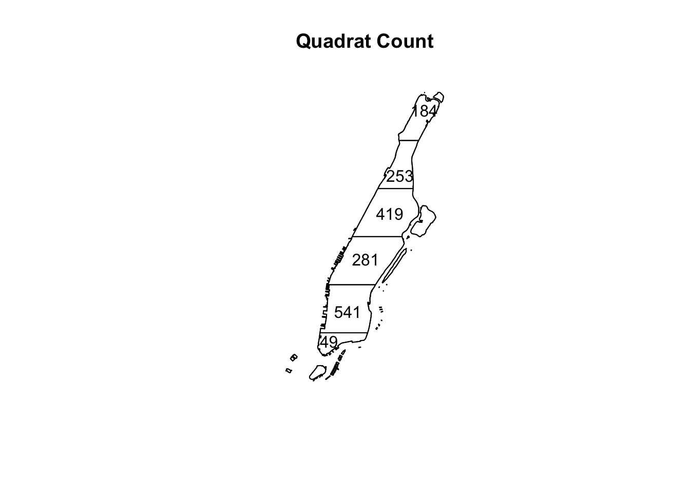
FIGURE 8.4: Count of burglaries in quadrats
As you can see with its irregular shape it is difficult to divide Manhattan in equally shaped and sized quadrats and thus it is hard to assess if regions of equal area contain a similar number of points. Notice, however,how the third quadrat from the bottom seems to have less incidents than the ones that surround it. A good portion of this quadrat is taken by Central Park, where you would not expect a burglary.
Instead, we can use other forms of tessellation, like hexagons by using the hextess() function (in spatstat). This is similar to the binning we introduced in Chapter 4, only using different functions. The numeric argument sets the size of the hexagons, you will need to play along to find an adequate value for your own applications. Rather than printing the numbers inside these hexagons (if you have many this will make it difficult to read in a plot) we can map a color to the intensity (the number of points per hexagon):
hex <- hextess(jitter_bur, 200)
q_hex <- quadratcount(jitter_bur, tess = hex)
plot(intensity(q_hex, image = TRUE), main = "Intensity map")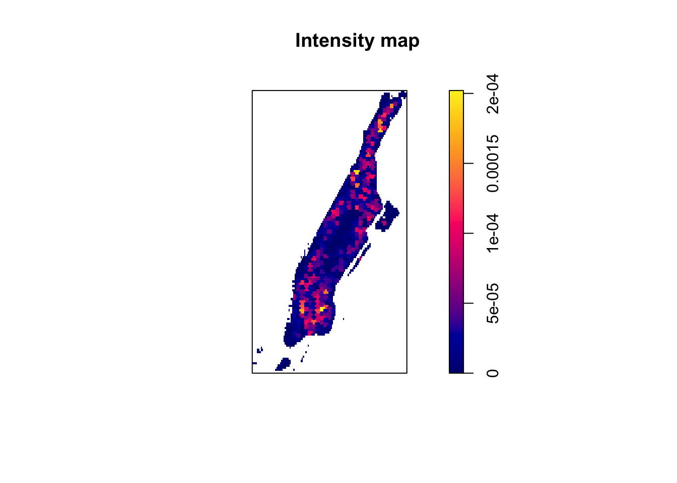
FIGURE 8.5: Intensity map of burglaries per hexagon
We can see more clearly now that areas of Manhattan, like Central Park, have understandably a very low intensity of burglaries, whereas others, like the Lower East Side and north of Washington Heights, have a higher intensity. So this map suggest to us that the process may not be homogeneous - hardly surprising when it comes to crime.
A key concept in spatial point pattern analysis is the idea of complete spatial randomness (or CSR for short). When we look at a point pattern process the first step in the process is to ask whether it has been generated in a random manner. Under CSR, points are (1) independent of each other (independence) and (2) have the same propensity to be found at any location (homogeneity).
We can generate data that conform to complete spatial randomness using the rpoispp() function (in spatstat). The r at the beginning is used to denote we are simulating data (you will see this is common in R) and we are using a Poisson point process, a good probability distribution for these purposes. Let’s generate 300 points in a random manner, and save this in the object poisson_ppp:
set.seed(1) # Use this seed to ensure you get the same results as us
poisson_ppp <- rpoispp(300)
We can plot this, to see how it looks
plot(poisson_ppp, main = "Complete Spatial Randomness")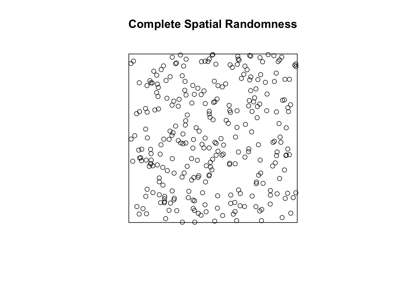
FIGURE 8.6: Simulated complete spatial randomness
You will notice that the points in a homogeneous Poisson process are not ‘uniformly spread’: there are empty gaps and clusters of points. This is very important. Random may look like what you may think non random should look. There seems to be places with apparent “clustering” of points. Keep this in mind when observing maps of crime distributions. Run the previous command a few times. You will see the map generated is different each time.
In classical literature, the homogeneous Poisson process (CSR) is usually taken as the appropriate ‘null’ model for a point pattern. Our basic task in analysing a point pattern is to find evidence against CSR. We can run a Chi Square test to check this in our data. So, for example, like we did above with Manhattan, we can split our area into quadrats.
q2 <- quadratcount(poisson_ppp, nx = 6, ny = 6)
plot(q2, main = "Quadrat Count")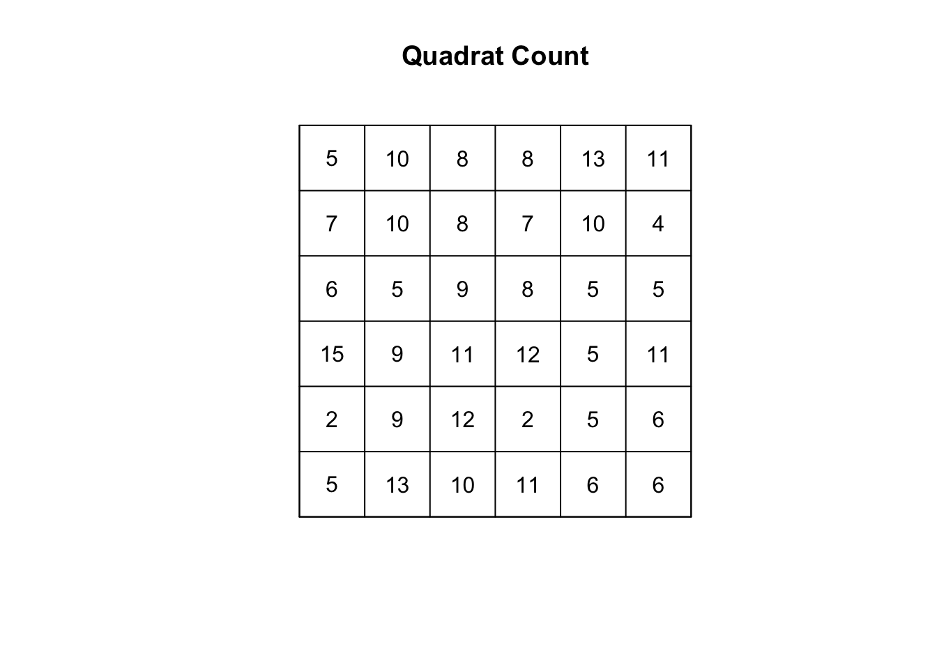
FIGURE 8.7: Count of our random points in quadrats
These numbers are looking more even than they did with our burglaries, but to really put this to the test, we run the Chi Square test using the quadrat.test() function.
quadrat.test(poisson_ppp, nx = 6, ny = 6)##
## Chi-squared test of CSR using quadrat counts
##
## data: poisson_ppp
## X2 = 44, df = 35, p-value = 0.3
## alternative hypothesis: two.sided
##
## Quadrats: 6 by 6 grid of tilesWe can see this p-value is greater than the conventional alpha level of 0.05 and therefore we cannot reject the null hypothesis that our point patterns come from complete spatial randomness - which is great news, as they indeed do!
How about our burglaries? Let’s run the quadrat.test() function to tell us whether burglaries in Manhattan follow spatial randomness.
quadrat.test(jitter_bur, nx = 1, ny = 6)##
## Chi-squared test of CSR using quadrat counts
##
## data: jitter_bur
## X2 = 238, df = 5, p-value <2e-16
## alternative hypothesis: two.sided
##
## Quadrats: 6 tiles (irregular windows)Observing the results we see that the p value is well below conventional standards for rejection of the null hypothesis. Observing our data of burglary in Manhattan would be extremely rare if the null hypothesis of a homogeneous distribution was true. We can then conclude that the burglary data is not randomly distributed in the observed space. But no cop nor criminologist would really question this. They would rarely be surprised by your findings! We do know, through research, that crime is not randomly distributed in space.
Beware as well that this test would come out as significant if the point pattern violates the property of independence between the points. It is important to keep in mind that the null may be rejected either because the process is not homogeneous or because the points are not independent, but the test doesn’t tell us the reason for the rejection. Equally, the power depend on the size of the quadrats (and they are not too large or too small). And the areas are not of equal size here in any case. So the test in many applications will be of limited use.
8.5 Mapping intensity estimates with spatstat
8.5.1 Basics of kernel density estimation (KDE)
One of the most common methods to visualise hot spots of crime, when we are working with point pattern data, is to use kernel density estimates. Kernel density estimation involves applying a function (known as a “kernel”) to each data point, which averages the location of that point with respect to the location of other data points. The surface that results from this model allows us to produce isarithmic maps. It is essentially a more sophisticated way of visualising intensity (points per area) than the tessellations we have covered so far.
Kernel density estimation maps are very popular among crime analysts. According to Chainey (2013a), 9 out of 10 intelligence professionals prefer it to other techniques for hot spot analysis. As compared to visualisations of crime that relies on point maps or thematic maps of geographic administrative units (such as LSOAs), kernel density estimation maps are considered best for location, size, shape and orientation of the hotspot. Chainey, Tompson, and Uhlig (2013) have also suggested that this method produces some of the best prediction accuracy. The areas identified as hotspots by KDE (using historical data) tend to be the ones that better identify the areas that will have high levels of crime in the future. Yet, producing these maps (as with any map, really) requires you to take a number of decisions that will significantly affect the resulting product and the conveyed message. Like any other data visualisation technique they can be powerful, but they have to be handled with great care.
Essentially this method uses a statistical technique (kernel density estimation) to generate a smooth continuous surface aiming to represent the intensity or volume of crimes across the target area. The technique, in one of its implementations (quartic kernel), is described in this way by Chainey (2013b):
- “a fine grid is generated over the point distribution;
- a moving three-dimensional function of a specified radius visits each cell and calculates weights for each point within the kernel’s radius. Points closer to the centre will receive a higher weight, and therefore contribute more to the cell’s total density value;
- and final grid cell values are calculated by summing the values of all kernel estimates for each location”
The values that we attribute to the cells in crime mapping will typically refer to the number of crimes within the area’s unit of measurement (intensity). Let’s produce one of this density maps, just with the default arguments of the density.ppp() function:
ds <- density.ppp(jitter_bur)
class(ds)
## [1] "im"The resulting object is of class im, a pixel image, a grid of spatial locations with values attached to them. You can visualise this image as a map (using plot()), contour plots (using contour()), or as a perspective plot (using persp()).
par(mfrow=c(1,3))
plot(ds, main='Pixel image')
contour(ds, main = 'Contour plot')
persp(ds, main = 'Perspective plot')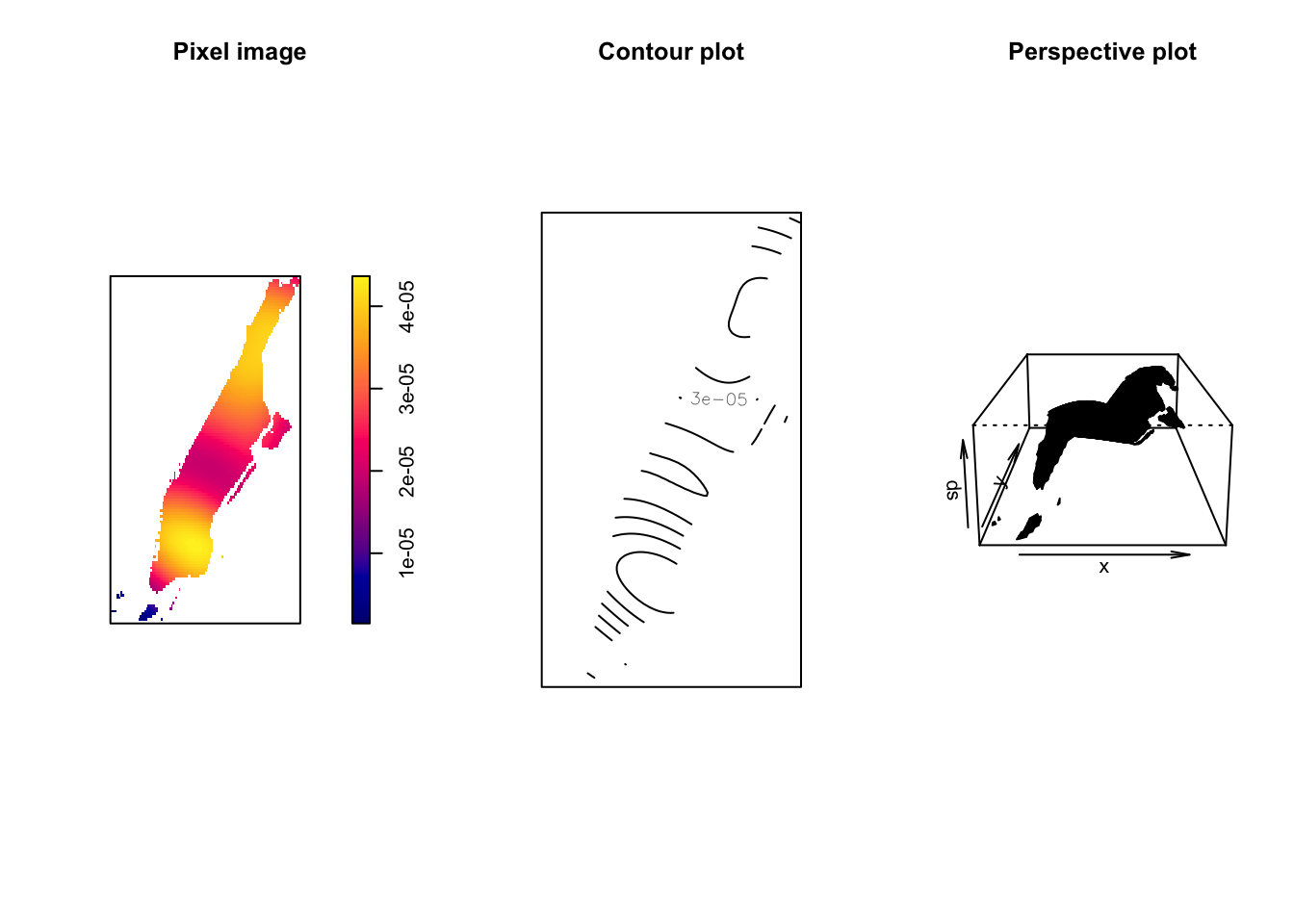
FIGURE 8.8: Visualisations of intensity of burglary in Manhattan
The density function is estimating a kernel density estimate. The result of density.ppp() is not a probability density. It is an estimate of the intensity function of the point process that generated the point pattern. The units of intensity are “points per unit area”. Density, in this context, is nothing but the number of points per unit area. This method computes the intensity continuously across the study area and the object returns a raster image. Depending what package you use to generate the estimation (e.g., spatstat, SpatialKDE, etc) you can set a different metric.
8.5.2 Selecting the appropriate bandwith for KDE
The defaults in density.ppp() are not necessarily the optimal ones for your application. When doing spatial density analysis there are a number of things you have to decide upon (e.g., bandwidth, kernel type, etc).
To perform this analysis we need to define the bandwidth of the density estimation, which basically determines the area of influence of the estimation. There is no general rule to determine the correct bandwidth; generally speaking if the bandwidth is too small the estimate is too noisy, while if bandwidth is too high the estimate may miss crucial elements of the point pattern due to oversmoothing. The key argument to pass to the density.ppp() is sigma=, which determines the bandwidth of the kernel. Sigma is the standard deviation of the kernel and you can enter a numeric value or a function that computes an appropriate value for it.
A great deal of research has been developed to produce algorithms that help in selecting the bandwidth (see Baddeley, Rubak, and Turner (2015) and Tilman Davies, Marshall, and Hazelton (2017) for details). In the spatstat package the functions bw.diggle(), bw.ppl(), and bw.scott() can be used to estimate the bandwidth according to difference methods (mean square error cross validation, likelihood cross validation, and Scott’s rule of thumb for bandwidth section in multidimensional smoothing respectively). The help files recommend the use of the first two. These functions run algorithms that aim to select an appropriate bandwidth.
set.seed(200) # We set this seed to ensure you get this same results when running
              # these algorithms
bw.diggle(jitter_bur)
## sigma
## 2.912bw.ppl(jitter_bur)## sigma
## 73.06bw.scott(jitter_bur)## sigma.x sigma.y
## 608.4 1447.6Scott’s rule generally provides larger bandwidth than the other methods. Don’t be surprised if your results do not match exactly the ones we provide if you do not use the same seed, the computation means that they will vary every time we run these functions. Keep in mind these values will be expressed in the unit of the projected coordinate system you use (in this case meters). We can visualise how they influence the appearance of ‘hot spots’:
set.seed(200)
par(mfrow=c(1,3))
plot(density.ppp(jitter_bur, sigma = bw.diggle(jitter_bur),edge=T),
     main = "Diggle")

plot(density.ppp(jitter_bur, sigma = bw.ppl(jitter_bur),edge=T),
     main="PPL")

plot(density.ppp(jitter_bur, sigma = bw.scott(jitter_bur) ,edge=T),
     main="Scott")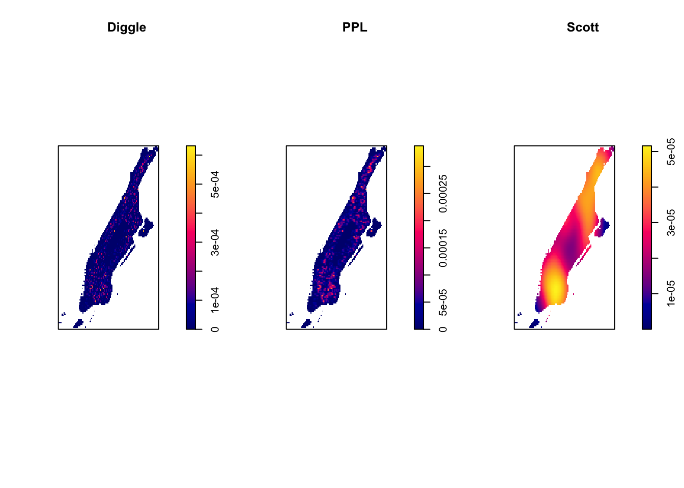
FIGURE 8.9: Kernel density maps with different bandwidth estimation algorightms
When looking for clusters, Baddeley, Rubak, and Turner (2015) suggest the use of the bw.ppl() algorithm because in their experience it tends to produce the more appropriate values when the pattern consists predominantly of tight clusters. But they also insist that if your purpose it to detect a single tight cluster in the midst of random noise then the bw.diggle() method seems to work best.
All these methods use a fixed bandwidth: they use the same bandwidth for all locations. As noted by Baddeley, Rubak, and Turner (2015) a “fixed smoothing bandwidth is unsatisfactory if the true intensity varies greatly across the spatial domain, because it is likely to cause oversmoothing in the high-intensity areas and undersmoothing in the low intensity areas” (p. 174). When using these methods in areas of high point density, the resulting bandwidth will be small, while in areas of low point density the resulting bandwidth will be large. This allow us to reduce smoothing in parts of the window where there are many points so that we capture more detail in the density estimates there, whilst at the same time increasing the smoothing in areas where there are less points.
With spatstat we can use an adaptive bandwidth method, were (1) a fraction of the points are selected at random and used to construct a tessellation; (2) a quadrat counting estimate of the intensity is produced; and (3) the process is repeated a set number of times and an average is computed. The adaptive.density() function (in spatstat) takes as arguments the fraction of points to be sampled (f) and the number of samples to be taken (nrep). The logical argument verbose when set to FALSE (not the default) means we won’t see a message in the console informing of the steps in the simulation.
plot(adaptive.density(jitter_bur, f=0.1, nrep=30, verbose=FALSE),
     main = "adaptive bandwidth method")
FIGURE 8.10: Adaptive bandwidth method for estimating bandwidth for KDE map
Which bandwidth to use? Chainey (2021) is critical of the various algorithms we have introduced. He suggests that “they tend to produce large bandwidths, and are considered unsuitable for exploring local spatial patterns of the density distribution of crime.” As we have seen with our example this is not necessarily the case, if anything both mean square error cross validation and likelihood cross validation produce small bandwidths in this example. When it comes to crime, Neville (2013) suggests that the “best choice would be to produce an interpolation that fits the experience of the department and officers who travel an area. Again, experimentation and discussions with beat officers will be necessary to establish which bandwidth choice should be used in future interpolations” (p. 10.22). This is generally accepted by other authors in the field. We see no damage in using these algorithms as a starting point and then, as suggested by most authors (see as well Chainey (2021)), to engage in a discussion with the direct users (considering what the map will be used for) to set in a particular bandwidth that is not too spiky, nor oversmoothed.
8.5.3 Selecting the smoothing kernel
Apart from selecting the bandwidth we also need to specify the particular kernel we will use. In density estimation there are different types of kernel. This relates to the type of kernel drawn around each point in the process of counting points around each point. The use of these functions will result in slightly different estimations. They relate to the way we weight points within the radius:
“The normal distribution weighs all points in the study area, though near points are weighted more highly than distant points. The other four techniques use a circumscribed circle around the grid cell. The uniform distribution weighs all points within the circle equally. The quartic function weighs near points more than far points, but the fall off is gradual. The triangular function weighs near points more than far points within the circle, but the fall off is more rapid. Finally, the negative exponential weighs near points much more highly than far points within the circle and the decay is very rapid.” (Levine 2013, chap. 10, p. 10).
Which one to use? Levine (2013) produces the following guidance: “The use of any of one of these depends on how much the user wants to weigh near points relative to far points. Using a kernel function which has a big difference in the weights of near versus far points (e.g., the negative exponential or the triangular) tends to produce finer variations within the surface than functions which weight more evenly (e.g., the normal distribution, the quartic, or the uniform); these latter ones tend to smooth the distribution more. However, Silverman (1986) has argued that it does not make that much difference as long as the kernel is symmetrical. Chainey (2013b) suggests that in his experience most crime mappers prefer the quartic function, since it applies greater weight to crimes closer to the centre of the grid. The authors of the CrimeStat workbook S. Smith and Bruce (2008), on the other hand, suggest that the choice of the kernel should be based in our theoretical understanding of the data generating mechanisms. By this they mean that the processes behind spatial dependence may be different according to various crime patterns and that this is something that we may want to take into account when selecting a particular function. They provide a table with some examples that may help you to understand what they mean. For example, for residential burglaries they recommend 1 mile with normally dispersed quartic or uniform interpolation, while for domestic violence 0.1 mile and tightly focused, negative exponential method (S. Smith and Bruce 2008).
The default kernel in density.ppp() is gaussian. But there are other options. We can use the epanechnikov, quartic or disc. There are also further options for customisation. We can compare these kernels, whilst using the ppl algorithm for sigma (remember we set seed at 200 for this particular value):
par(mfrow=c(2,2))
# Gaussian kernel function (the default)
plot(density.ppp(jitter_bur, sigma = bw.ppl(jitter_bur), edge=TRUE), main="Gaussian")

# Epanechnikov (parabolic) kernel function
plot(density.ppp(jitter_bur, kernel = "epanechnikov", sigma = bw.ppl(jitter_bur),
                 edge=TRUE), main="epanechnikov")

# Quartic kernel function
plot(density.ppp(jitter_bur, kernel = "quartic", sigma = bw.ppl(jitter_bur), edge=TRUE),
     main="Quartic")

plot(density.ppp(jitter_bur, kernel = "disc", sigma = bw.ppl(jitter_bur), edge=TRUE),
     main="Disc")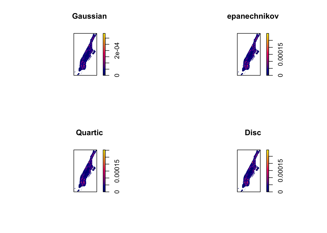
FIGURE 8.11: KDE maps created with different kernel shapes
You can see how the choice of the kernel has less of an impact than the choice of the bandwidth. In practical terms choice of the specific kernel is of secondary importance to the bandwidth.
Equally, you may have noticed an argument in density.ppp() we have not discussed edge = TRUE. What is this? When estimating the density we are not observing points outside our window. In the case of an island like Manhattan perhaps this is not an issue. But often when computing estimates for a given jurisdiction we need to think about what is happening in the jurisdiction next door to us. Our algorithm does not see the crimes in jurisdiction neighbouring ours and so the estimation around the edges of our boundaries receive fewer contributions in the computation. By setting edge = TRUE we are effectively applying a correction that tries to compensate for this negative bias.
8.5.4 Weighted kernel density estimates
In the past examples we used the un-weighted version of the estimation methods, but if the points are weighted (like for example by multiplicity) we can use weighted versions of these methods. We simply need to pass an argument that specifies the weights.
set.seed(200)
plot(density.ppp(bur_ppp_m, sigma = bw.ppl(bur_ppp_m), edge = T,
                 kernel = "quartic", weights = marks(bur_ppp_m)),
     main = "Weighted Points")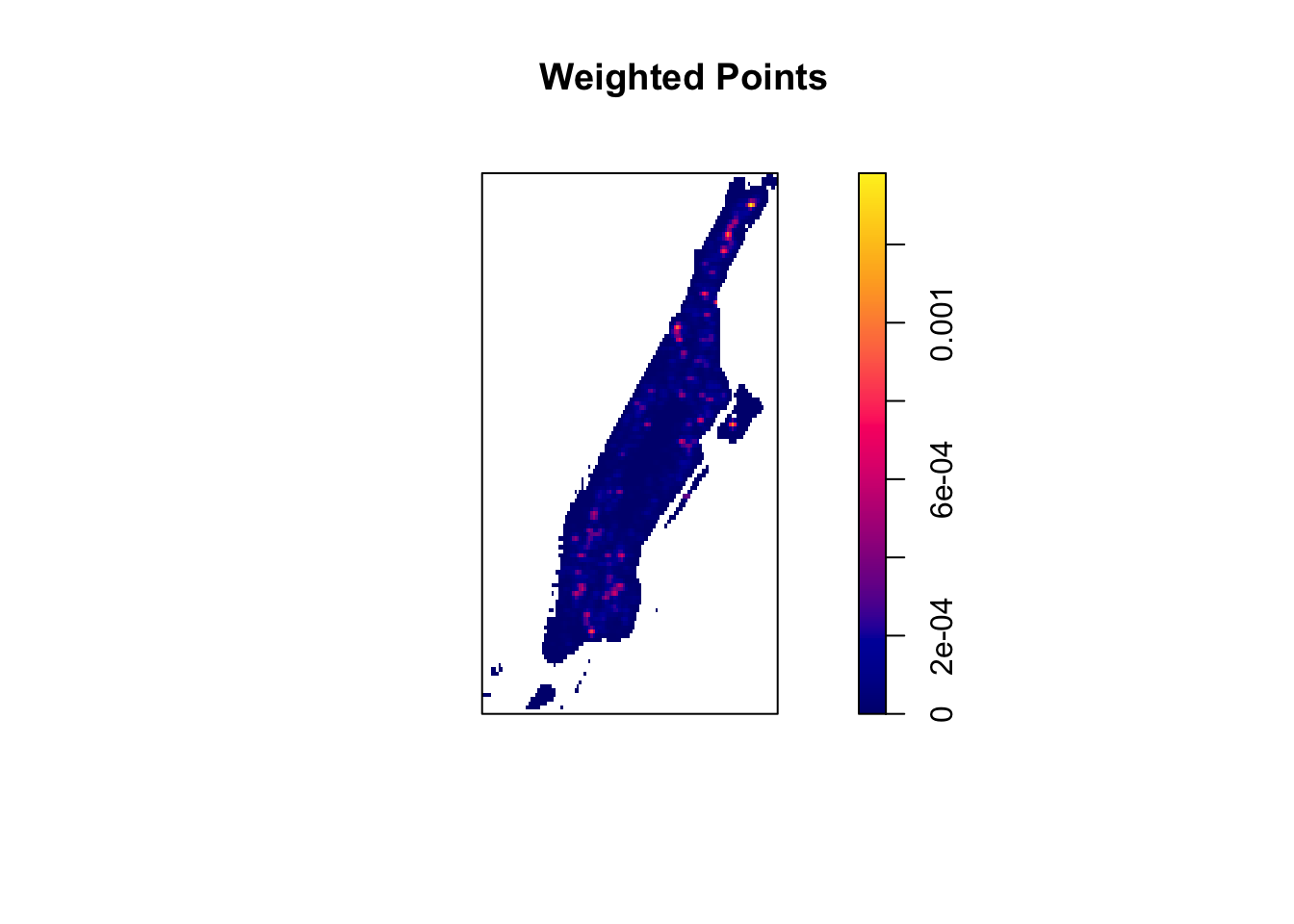
FIGURE 8.12: Weighting KDE estimates
8.5.5 Better KDE maps using leaflet
The plots produced by spatstat are good for initial exploration, but if you want to present this to an audience you may to use one of the various packages we have covered so far for visualising spatial data. Here we show how to use leaflet for ploting densities. Hot spot analysis often have an exploratory character and the interactivity provided by leaflet is particularly helpful, since it allow us to zoom in and out and check the details of the areas with high intensities.
Often it is convenient to use a basemap to provide context. In order to do that we first need to turn the image object generated by the spatstat package into a raster object, a more generic format for raster image used in R. Remember rasters from the first chapter? Now we finally get to use them a bit! First we store the density estimates produced by density.ppp() into an object (which will be of class im, a two dimensional pixel image) and then using the raster() function from the raster package we generate a raster object.
set.seed(200)
dmap1 <- density.ppp(jitter_bur, kernel = "quartic", sigma = bw.ppl(jitter_bur), edge=T)
# create raster object from im object
r1 <- raster(dmap1)
# plot the raster object
plot(r1, main = "Raster")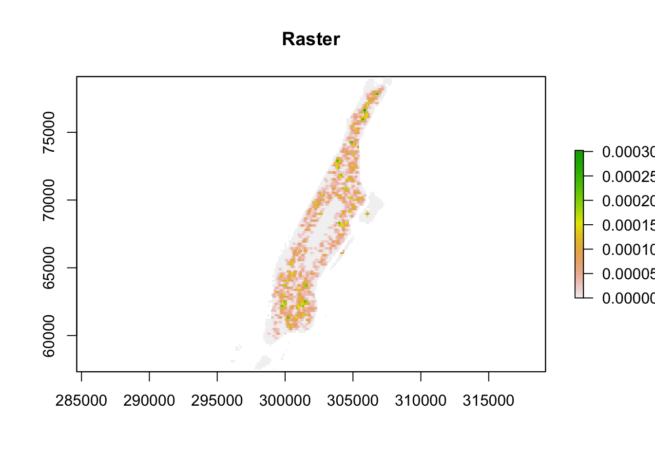
FIGURE 8.13: Raster image of KDE output
We can remove the areas with very low density of burglaries for better reading of the map:
#remove very low density values
r1[r1 < 0.00010 ] <- NA

#multiply by 1000 to re-express intensity in terms of burglaries per km
values(r1) <- values(r1)*1000
Now that we have the raster we can add it to a basemap. Two-dimensional RasterLayer objects (from the raster package) can be turned into images and added to Leaflet maps using the addRasterImage() function. The addRasterImage() function works by projecting the RasterLayer object to EPSG:3857 and encoding each cell to an RGBA color, to produce a PNG image. That image is then embedded in the map widget. This is only suitable for small to medium sized rasters.
It’s important that the RasterLayer object is tagged with a proper coordinate reference system, so that leaflet can then reproject to EPSG:3857. Many raster files contain this information, but some do not. Here is how you would tag a raster layer object r1 which contains the EPSG:32118 data:
#make sure we have right CRS, which in this case is the New York 32118

crs(r1) <- "EPSG:32118"
The way we assign the CRS above is using the now most accepted PROJ6 format. You can find how these different formats apply to each coordinate system in the spatialreference.org online archive.
Now we are ready to plot, although first we will create a more suitable colour palette and, since the values in the scale are quite close to 0 will multiple by a constant, to make the labels more readable. For this we use the values() function from the raster package that allows us to manipulate the values in a raster object:
pal <- colorNumeric("Reds", values(r1),
  na.color = "transparent") #Create color palette

#and then make map!
leaflet() %>%
  addTiles() %>%
  addProviderTiles(providers$Stamen.TonerLite) %>%
  addRasterImage(r1, colors = pal, opacity = 0.7) %>%
  addLegend(pal = pal, values = values(r1),
    title = "Burglary map")
FIGURE 8.14: Leaflet map for exploring KDE layer of burglaries in Manhattan
And there you have it. Perhaps those familiar with Manhattan have some guesses as to what may be going on there?
8.5.6 Problems with KDE
There are at least two problems with these maps. First, they are just a convenient visualisation to represent the location of crime incidents. But they are not adjusting by the population at risk. If all you care is where most crimes are taking place, that may then be ok. But if you are interested in relative risk, intensity adjusting by population at risk, then you are bound to be misled by these methods, which usually will plot very well the distribution of the population at risk. Second, the Poisson process, as we saw, creates what may appear as areas with more points than others, even though it is a random process. In other words, you may just be capturing random noise with these maps.
There are a number of ways to adjust for background population at risk when producing density estimates. Many of these methods have been developed in spatial epidemiology. In criminology, the population at risk is generally available only at more aggregated (at some census geography level) than in many of those applications (where typically you have points representing individuals without a disease being contrasted with points representing individuals with a disease). So, although one could extract the centroids of these polygons representing census tracts or districts as points and mark them with a value (say population count or number of housing units), there isn´t a great advantage to go to all this trouble. In fact by locating all the mass of the population at risk in the centroids of the polygons you are introducing some distortion. So if you want to adjust for the population at risk, it is probably better to map out rates in the ways we described in previous chapters. We just need to be aware, then, that KDE surfaces in essence are simply mapping counts of crime. We therefore need to interpret density maps with this very significant caveat.
The other problem we had is that a Poisson process under CSR can still result in a map that one could read as identifying hot spots, whereas all we have is noise. Remember the poisson_ppp object we created earlier, which demonstrated complete spatial randomness? Well, if we were that way inclined, we could easily compute a KDE for this:
set.seed(200)

plot(density.ppp(poisson_ppp, kernel = "quartic", sigma = bw.diggle(poisson_ppp),
                 edge=T), main = "KDE for random poisson point process")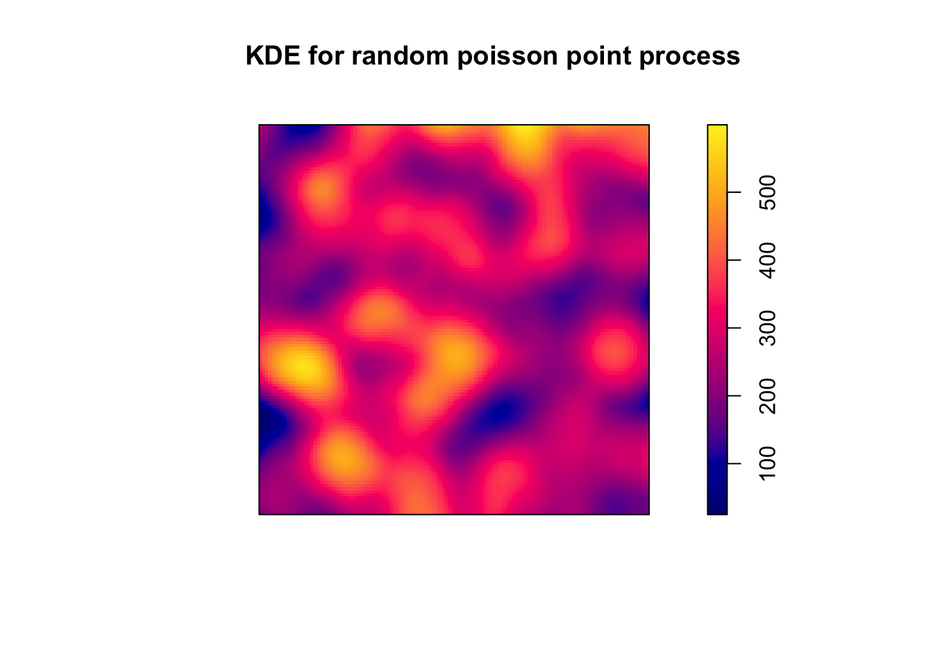
FIGURE 8.15: Kernel density map for quartic kernel
And there you go, you could come to the view looking at this density map that the intensity is driven by some underlying external risk factor when in fact the process is purely random. In subsequent chapters we will learn about methods that can be used to ensure we don’t map out hot spots that may be the product of random noise.
8.5.7 Other packages for KDE
In this chapter we have focused on spatstat for it provides a comprehensive suite of tools for working with spatial point patterns. The snippets of code and examples we have used here only provide a superficial glimpse into the full potential of this package. But spatstat is by no means the only package that can be used for generating spatial density estimates. We need to mention at least two alternatives: SpatialKDE and sparr.
SpatialKDE implements kernel density estimation for spatial data with all the required settings, including the selection of bandwidth, kernel type, and cell size (which was computed automatically by density.ppp()). It is based in an algorithm used in QGIS, the best free GIS system relying primarily on a point and click interface. Unlike spatstat, SpatialKDE can work with sf objects. But it also finds it more convenient to have the data on a projected coordinate systems, so that it can compute distances on metres rather than with decimal degrees.
The package sparr focuses on methods to compare densities and thus estimate relative risk, even at a spatiotemporal scale. It is written in such a way as to allow compatibility with spatstat. The basic functionality allows to estimate KDE maps through the bivariate.density() function. This function can take a ppp object and produce a KDE map. In some ways it gives the analyst more flexibility than density.ppp(): allowing to modulate the resolution of the grid, allows for two different methods to control for edge effects, the type of estimate produced (intensity or density, that integrates to 1), etc. This package also introduces various methods for estimating the bandwidth different to those existing in spatstat. Critically, it introduces a function that allows for spatiotemporal kernel density estimation: spattemp.density(). For more details see the help files for sparr, and the tutorial by Tilman Davies, Marshall, and Hazelton (2017).
8.6 Summary and further reading
For a deeper understanding of the issues discussed here we recommend the following reading. The documentation manual for CrimeStat (Chapter 10) has a detailed technical discussion of density estimation that is suited for crime analysts (Levine 2013). Other manuals written for crime analysts also provide appropriate introductions Gorr and Kurland (2012). Chapter 7 of Bivand, Pebesma, and Gómez-Rubio (2013) also provides a good introduction to spatial pattern analysis with R. For a fuller coverage of this kind of analysis with R, nothing can replace Baddeley, Rubak, and Turner (2015). This book, at 810 pages, is dedicated to spacestat and it provides a comprehensive discussion of spatial pattern analysis well beyond what we cover in this chapter. For a discussion of alternatives to KDE so that the method do not assign probabilities of occurrence where this is not feasible see Woodworth et al. (2014) (though beware this has not yet being implemented into R). In the next chapter we will discover much of what we have learnt in this one has to be adapted when working with crime data, for this data typically only appears along street networks.