Chapter 12 Spatial regression models
12.1 Introduction
In science one of our main concerns is to develop models of the world, models that help us to understand the world a bit better or to predict how things will develop better. Crime analysis also is interested in understanding the processes that may drive crime. This is a key element in the SARA process (analysis) that form part of the problem oriented policing approach (Eck and Spelman 1997). Statistics provides a set of tools that help researchers build and test scientific models, and to develop predictions. Our models can be simple. We can think that unemployment is a factor that may help us to understand why cities differ in their level of violent crime. We could express such a model like this:

FIGURE 12.1: A simple model
Surely we know the world is complex and likely there are other things that may help us to understand why some cities have more crime than others. So, we may want to have tools that allow us to examine such models. Like, for example, the one below:
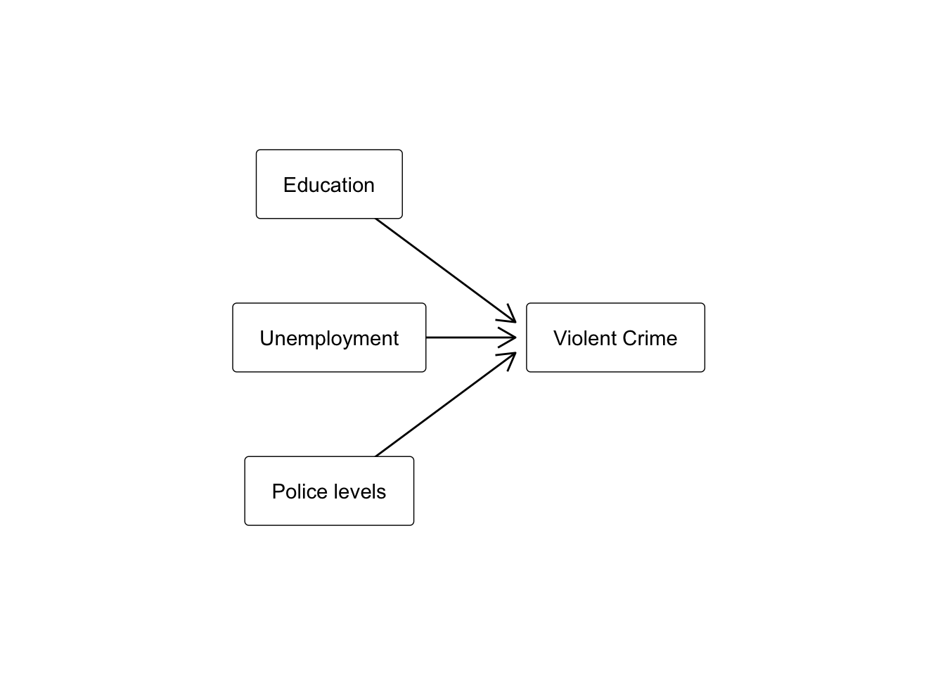
FIGURE 12.2: A slightly less simple model
In this chapter we cover regression analysis for spatial data, a key tool for testing models. Regression is a flexible technique that allows you to “explain” or “predict” a given outcome, variously called your outcome, response or dependent variable, as a function of a number of what is variously called inputs, features or independent, explanatory, or predictive variables. We assume that you have covered regression analysis in previous training. If that is not the case or you want a quick refresher, we suggest you consult Appendix B: Regression analysis (a refresher) in the website for this book. Our focus in this chapter will be in a series of regression models that are appropriate when your data has a spatial structure.
There is a large and developing field, spatial econometrics, dedicated to develop this kind of models. Traditionally these models were fit using maximum likelihood, whereas in the last few years we have seen the development of new approaches. There has also been some parallel developments in different disciplines, some of which have emphasised simultaneous autoregressive models and others (such as disease mapping) that have emphasised conditional autoregressive models. If these terms are not clear, do not worry, we will come back to them later on. This is a practical R focused introductory text and, therefore, we cannot cover all the nuisance associated with some of these differences and the richness of spatial econometrics. Here we will just simply introduce some of the key concepts and more basic models for cross sectional spatial data, illustrate them through a practical example, and later on will provide guidance to more in depth literature.
We need to load the libraries we will use in this chapter. Although there are various packages that can be used to fit spatial regression models, particularly if you are willing to embrace a Bayesian approach, our focus in this chapter will be on spatialreg. This package contains the estimation functions for spatial cross sectional models that before were shipped as part of spdep, sphet, and spse. There are various ways of thinking about spatial regression, here we will focus in those that rely on frequentist methods and a spatial weight matrix (to articulate the spatial nature of the data).
# Packages for handling spatial data and for geospatial carpentry
library(sf)
library(sp)
library(spdep)
# Packages for regression and spatial regression
library(arm)
library(effects)
library(spatialreg)
# Packages for mapping and visualisation
library(tmap)
library(ggplot2)
# Packages with spatial datasets
library(geodaData)
Here we will return to the “ncovr” data we have used in previous chapters. This dataset was produced as part of the National Consortium on Violence Research (NCOVR) agenda, a National Science Foundation initiative that was led by Al Blumstein. A piece of work that resulted from this initiative was the paper led by Robert Baller in Criminology, for which this data was compiled (Baller et al. 2001). This paper co-authored by Luc Anselin, one of the key figures in the field of spatial econometrics, run and describes spatial regression models of the kind we cover in this chapter with this dataset. It would be helpful, thus, to read that piece in parallel to this chapter.
data("ncovr")12.2 Challenges for regression with spatial data
There are a number of issues when it comes to fitting regression with spatial data. We will highlight three: validity, spatial dependence, and spatial heterogeneity. One, validity, is common to regression in general, although with spatial data it acquires particular relevance. The other two (spatial dependence and spatial heterogeneity) are typical of spatial data.
The most important assumption of regression is that of validity. The data should be appropriate for the question that you are trying to answer. As noted by Gelman and Hill (2007):
“Optimally, this means that the outcome measure should accurately reflect the phenomenon of interest, the model should include all relevant predictors, and the model should generalize to all cases to which it will be applied… Data used in empirical research rarely meet all (if any) of these criteria precisely. However, keeping these goals in mind can help you be precise about the types of questions you can and cannot answer reliably”
Although validity is a key assumption for regression, whether spatial or not, it is the case that the features of spatial data make it particularly challenging (as discussed in detail by Haining (2003)).
The second challenge is spatial dependence. A key assumption of regression analysis is the independence between the observations. That is, a regression model is formally assuming that what happens in area \(X_i\) is not in any way related (it is independent) of what happens in area \(X_{ii}\). But if those two areas are adjacent or proximal in geographical space we know that there is a good chance that this assumption may be violated. Values that are close together in space are unlikely to be independent. Crime levels, for example, tend to be similar in areas that are close to each other. The problem for regression is not so much autocorrelation in the response or dependent variable, but the remaining autocorrelation in the residuals. If the spatial autocorrelation of our outcome \(y\) is fully accounted by the spatial structure of the observed predictor variables in our model, we don´t really have a problem. On the other hand, when the residuals of your model display spatial autocorrelation you are violating an assumption of the standard regression model, and you need to find a solution for this.
When positive spatial autocorrelation is observed, using a regression model that assumes independent errors will lead to an underestimation of the uncertainty around your parameters (or overestimation if the autocorrelation is negative). With positive spatial autocorrelation you will be more likely to engage in a Type I error (concluding the coefficient for a given predictor is not zero when this decision is not justified). Essentially, we have less degrees of freedom, as Haining and Li (2020) notes for positive spatial autocorrelation (the most common case in crime analysis and social science):
“Underlying the results… is the fact that ´less information´ about the parameter of interest… is contained in a dataset where observations are positively autocorrelated… The term ´effective´ sample size has been coined and used to measure the information content in a set of autocorrelated data. Compared with the case of N independent observations, if we have N autocorrelated data values then the effective sample size is less than N (how much less depends on how strongly autocorrelated values are). The effective sample size can be thought of as the equivalent number of independent observations available for estimating the parameter… It is this reduction in the information content of the data that increases the uncertainty of the parameter estimate… This arises because each observation contains what might call ´overlapping´ or ´duplicate´ information about other observations” (p. 7)
In previous weeks we covered formal tests for spatial autocorrelation, which allow us to test whether this is a feature of our dependent (or predictor) variable. So before we fit a regression model with spatial data we need to explore the issue of autocorrelation in the attributes of interest, but critically what we need to establish is whether there is spatial autocorrelation in the residuals. In this session, we will see that there are two basic ways of adjusting for spatial autocorrelation: through a spatial lag model or through a spatial error model. Although there are multiple types of spatial regression models (see Anselin and Rey (2014), Bivand, Millo, and Piras (2021), Chi and Zhu (2020), and Beale et al. (2010), specifically for a review of their relative performance), these are the two basic forms that you probably (particularly if your previous statistical training sits in the frequentist tradition) need to understand before you get into other types.
A third challenge for regression models with spatial data is spatial heterogeneity (also referred to as non-stationarity). We already discussed the concept of spatial homogeneity when introducing the study of point patterns. In that context we defined spatial homogeneity as the homogeneous intensity of the point pattern across the study surface. But spatial homogeneity is a more general concept that applies to other statistical properties. In the context of lattice or area level data it may refer to the mean value of an attribute (such as crime rate) across areas but it could also refer to how other variables are related to our outcome of interest across the study region. It could be the case, for example, that some predictors display spatial structure in how they affect the outcome. It could be, for example, that presence of licensed premises to sell alcohol have a different impact on the level of violent crime in different types of communities in our study region. If there is spatial heterogeneity in these relationships we need to account for it. We could deal with this challenge through some form of data partition, spatial regime, or local regression model (where we allow the regression coefficient to be area specific) such as geographically weighted regression. We will discuss this third challenge to regression in greater detail in the next chapter.
Not so much a challenge but an important limitation is the presence of missing data. Unlike in standard data analysis where you have a sample of \(n\) observations and there are a number of approaches to impute missing data. In the context of spatial econometrics, you only have one realisation of the data generating mechanism. As such, if there is missing data for some of the areas, the models cannot be estimated, although some solutions have been proposed when the percentage of missing cases is very small (see Floch and LeSaout (2018)).
In general, the development of a spatial regression model requires taking into account these challenges. There are various aspects that building the model will require (Kopczewska 2021); selecting the right model for the data at hand, the estimation method, and the model specification (variables to include).
12.3 Fitting a non-spatial regression model with R
The standard approach traditionally was to start with a non-spatial linear regression model and then to test whether or not this baseline model needs to be extended with spatial effects (Elhorst 2014). Given we need to check autocorrelation in residuals, part of the workflow for modelling through regression spatial data will involve fitting a non spatial regression model. In order to fit the model we use the stats::lm() function using the formula specification (Y ~ X). Typically you want to store your regression model in a “variable”, let’s call it “fit1_90”. Here we model homicide rate in the 1990s (HR90) using, to start with, just two variables of interest, RD90- Resource Deprivation/Affluence, and SOUTH - Counties in the southern region scored 1.
ncovr$SOUTH_f <- as.factor(ncovr$SOUTH) # specify this is a categorical variable
fit1_90 <- lm(HR90 ~ RD90 + SOUTH_f, data=ncovr)
You will see in your R Studio global environment space that there is a new object called fit1_90 with 13 elements on it. We can get a sense for what this object is and includes using the functions we introduced in previous weeks:
class(fit1_90)
attributes(fit1_90)
R is telling us that this is an object of class lm and that it includes a number of attributes. One of the beauties of R is that you are producing all the results from running the model, putting them in an object, and then giving you the opportunity for using them later on. If you want to simply see the basic results from running the model you can use the standard summary() function.
summary(fit1_90)##
## Call:
## lm(formula = HR90 ~ RD90 + SOUTH_f, data = ncovr)
##
## Residuals:
## Min 1Q Median 3Q Max
## -16.48 -3.00 -0.58 2.22 68.15
##
## Coefficients:
## Estimate Std. Error t value Pr(>|t|)
## (Intercept) 4.727 0.139 33.9 <2e-16 ***
## RD90 2.965 0.111 26.8 <2e-16 ***
## SOUTH_f1 3.181 0.222 14.3 <2e-16 ***
## ---
## Signif. codes:
## 0 '***' 0.001 '**' 0.01 '*' 0.05 '.' 0.1 ' ' 1
##
## Residual standard error: 5.3 on 3082 degrees of freedom
## Multiple R-squared: 0.365, Adjusted R-squared: 0.364
## F-statistic: 884 on 2 and 3082 DF, p-value: <2e-16The coefficients suggest that, according to our fitted model, when comparing two counties with the same level of resource deprivation, the homicide rate on average will be about 3 points higher in the Southern counties than in the Northern counties. And when comparing counties “adjusting” for their location, the homicide rate will be also around 3 points higher for every one unit increase in the measure of resource deprivation. Although it is tempting to talk of the “effect” of these variables in the outcome (homicide rate), this can mislead yourself and your reader about the capacity of your analysis to establish causality, so it is safer to interpret regression coefficients as comparisons (Gelman, Hill, and Vehtari 2020).
With more than one input, you need to ask yourself whether all of the regression coefficients are zero. This hypothesis is tested with a F test. Again we are assuming the residuals are normally distributed, though with large samples the F statistics approximates the F distribution. You see the F test printed at the bottom of the summary output and the associated p value, which in this case is way below the conventional .05 that we use to declare statistical significance and reject the null hypothesis. At least one of our inputs must be related to our response variable. Notice that the table printed also reports a t test for each of the predictors. These are testing whether each of these predictors is associated with the response variable when adjusting for the other variables in the model. They report the “partial effect of adding that variable to the model” (James et al. 2013: 77). In this case we can see that all inputs seem to be significantly associated with the output.
The interpretation or regression coefficients is sensitive to the scale of measurement of the predictors. This means one cannot compare the magnitude of the coefficients to compare the relevance of variables to predict the response variable. One way of dealing with this is by rescaling the input variables. A common method involves subtracting the mean and dividing by the standard deviation of each numerical input. The coefficients in these models is the expected difference in the response variable, comparing units that differ by one standard deviation in the predictor while adjusting for other predictors in the model. Instead, Gelman (2008) has proposed dividing each numeric variables by two times its standard deviation, so that the generic comparison is with inputs equal to plus/minus one standard deviation. As Gelman explains the resulting coefficients are then comparable to untransformed binary predictors. The implementation of this approach in the arm package subtract the mean of each binary input while it subtract the mean and divide by two standard deviations for every numeric input. The way we would obtain these rescaled inputs uses the standardize() function of the arm package, that takes as an argument the name of the stored fit model.
standardize(fit1_90)##
## Call:
## lm(formula = HR90 ~ z.RD90 + c.SOUTH_f, data = ncovr)
##
## Coefficients:
## (Intercept) z.RD90 c.SOUTH_f
## 6.18 5.93 3.18Notice the main change affects the numerical predictors. The unstandardised coefficients are influenced by the degree of variability in your predictors, which means that typically they will be larger for your binary inputs. With unstandardised coefficients you are comparing complete change in one variable (whether one is a Southern county or not) with one-unit changes in your numerical variable, which may not amount to much change. So, by putting in a comparable scale, you avoid this problem. Standardising in the way described here will help you to make fairer comparisons. This standardised coefficients are comparable in a way that the unstandardised coefficients are not. We can now see what inputs have a comparatively stronger effect. It is very important to realise, though, that one should not compare standardised coefficients across different models.
In the social sciences there is a great interest in what are called conditional hypothesis or interactions. Many of our theories do not assume simply additive effects but multiplicative effects. For example, you may think that a particular crime prevention programme may work in some environments but not in others. The interest in this kind of conditional hypothesis is growing. One of the assumptions of the regression model is that the relationship between the response variable and your predictors is additive. That is, if you have two predictors \(x_1\) and \(x_2\). Regression assumes that the effect of \(x1\) on \(y\) is the same at all levels of \(x_2\). If that is not the case, you are then violating one of the assumptions of regression. This is in fact one of the most important assumptions of regression, even if researchers often overlook it.
One way of extending our model to accommodate for interaction effects is to add additional terms to our model, a third predictor \(x_3\), where \(x_3\) is simply the product of multiplying \(x_1\) by \(x_2\). Notice we keep a term for each of the main effects (the original predictors) as well as a new term for the interaction effect. “Analysts should include all constitutive terms when specifying multiplicative interaction models except in very rare circumstances” (Brambor, Clark, and Golder 2006: 66).
How do we do this in R? One way is to use the following notation in the formula argument. Notice how we have added a third term RD90:SOUTH_f, which is asking R to test the conditional hypothesis that resource deprivation may have a different impact on homicide for southern and northern counties.
fit2_90 <- lm(HR90 ~ RD90 + SOUTH_f + RD90:SOUTH_f , data=ncovr)
# which is equivalent to:
# fit_2 <- lm(HR90 ~ RD90 * SOUTH_f , data=ncovr)
summary(fit2_90)
##
## Call:
## lm(formula = HR90 ~ RD90 + SOUTH_f + RD90:SOUTH_f, data = ncovr)
##
## Residuals:
## Min 1Q Median 3Q Max
## -17.05 -3.00 -0.57 2.23 68.14
##
## Coefficients:
## Estimate Std. Error t value Pr(>|t|)
## (Intercept) 4.548 0.159 28.68 <2e-16 ***
## RD90 2.581 0.196 13.15 <2e-16 ***
## SOUTH_f1 3.261 0.225 14.51 <2e-16 ***
## RD90:SOUTH_f1 0.562 0.238 2.37 0.018 *
## ---
## Signif. codes:
## 0 '***' 0.001 '**' 0.01 '*' 0.05 '.' 0.1 ' ' 1
##
## Residual standard error: 5.29 on 3081 degrees of freedom
## Multiple R-squared: 0.366, Adjusted R-squared: 0.365
## F-statistic: 592 on 3 and 3081 DF, p-value: <2e-16You see here that essentially you have only two inputs (resource deprivation and south) but several regression coefficients. Gelman and Hill (2007) suggest reserving the term input for the variables encoding the information and to use the term predictor to refer to each of the terms in the model. So here we have two inputs and three predictors (one for SOUTH, another for resource deprivation, and a final one for the interaction effect). In this case the test for the interaction effect is significant, which suggests there may be such an interaction. Let’s visualise the results with the effects package:
plot(allEffects(fit2_90), ask=FALSE)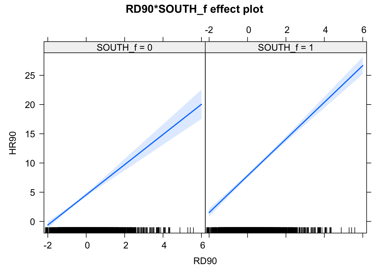
FIGURE 12.3: Effect plots for effect of South variable on relationship between homicide rate and resource deprivation
Notice that essentially what we are doing is running two regression lines and testing whether the slope is different for the two groups. The intercept is different, we know that Southern counties are more violent, but what we are testing here is whether the level of homicide goes up in a steeper fashion (and in the same direction) for one or the other group as the level of resource deprivation goes up. We see that’s the case here. The estimated lines are almost parallel, but the slope is a bit steeper in the Southern counties. In Southern counties resource deprivation seems to have more of an impact on homicide than in Northern counties. This is related to one of the issues we raised earlier regarding spatial regression, that of hetereogeneity. Here what we see is that there some evidence of non-stationarity in the relationship between our predictors and our outcome.
A word of warning about interactions, the moment you introduce an interaction effect the meaning of the coefficients for the other predictors changes (what it is often referred as to the “main effects” as opposed to the interaction effect). You cannot retain the interpretation we introduced earlier. Now, for example, the coefficient for the SOUTH variable relates the marginal effect of this variable when RD90 equals zero. The typical table of results helps you to understand whether the effects are significant but offers little of interest that will help you to meaningfully interpret what the effects are. For this is better you use some of the graphical displays we have covered.
Essentially what happens is that the regression coefficients that get printed are interpretable only for certain groups. So now:
The intercept still represents the predicted score of homicide for southern counties and have a score of 0 in resource deprivation (as before).
The coefficient of SOUTH_f1 now can be thought of as the difference between the predicted score of homicide rate for northern counties that have a score of 0 in resource deprivation and northern counties that have a score of 0 in resource deprivation.
The coefficient of RD90 now becomes the comparison of mean homicide rate for Southern counties who differ by one point in resource deprivation.
The coefficient for the interaction term represents the difference in the slope for RD90 comparing Southern and Northern counties, the difference in the slope of the two lines that we visualised above.
Models with interaction terms are too often misinterpreted. We strongly recommend you read Brambor, Clark, and Golder (2006) to understand some of the issues involved.
12.4 Looking at the residuals and testing for spatial autocorrelation in regression
Residuals measure the distance between our observed Y values, \(Y\), and the predicted Y values, \(\hat{Y}\). So in essence they are deviations of observed reality from your model. Your regression line (or hyperplane in the case of multiple regression) is optimised to be the one that best represent your data if the assumptions of the model are met. Residuals are very helpful to diagnose, then, whether your model is a good representation of reality or not. Most diagnostics of the assumptions for regression rely on exploring the residuals.
Now that we have fitted the model we can extract the residuals. If you look at the “fit_1” object in your RStudio environment or if you run the str() function to look inside this object you will see that this object is a list with different elements, one of which is the residuals. An element of this object then includes the residual for each of your observations (the difference between the observed value and the value predicted by your model). We can extract the residuals using the residuals() function and add them to our spatial data set. Let´s fit a model with all the key predictors available in the dataset and inspect the residuals.
# write model into object to save typing later
eq1_90 <- HR90 ~ RD90 + PS90 + MA90 + DV90 + UE90 + SOUTH_f
fit3_90 <- lm(eq1_90, data=ncovr)
summary(fit3_90)
##
## Call:
## lm(formula = eq1_90, data = ncovr)
##
## Residuals:
## Min 1Q Median 3Q Max
## -17.64 -2.61 -0.70 1.65 68.51
##
## Coefficients:
## Estimate Std. Error t value Pr(>|t|)
## (Intercept) 6.5165 1.0240 6.36 2.3e-10 ***
## RD90 3.8723 0.1427 27.13 < 2e-16 ***
## PS90 1.3529 0.1003 13.49 < 2e-16 ***
## MA90 -0.1011 0.0274 -3.69 0.00023 ***
## DV90 0.5829 0.0545 10.69 < 2e-16 ***
## UE90 -0.3059 0.0409 -7.47 1.0e-13 ***
## SOUTH_f1 2.1941 0.2205 9.95 < 2e-16 ***
## ---
## Signif. codes:
## 0 '***' 0.001 '**' 0.01 '*' 0.05 '.' 0.1 ' ' 1
##
## Residual standard error: 4.99 on 3078 degrees of freedom
## Multiple R-squared: 0.436, Adjusted R-squared: 0.435
## F-statistic: 397 on 6 and 3078 DF, p-value: <2e-16ncovr$res_fit3 <- residuals(fit3_90)If you now look at the dataset you will see that there is a new variable with the residuals. In those cases where the residual is negative this is telling us that the observed value is lower than the predicted (that is, our model is overpredicting the level of homicide for that observation) when the residual is positive the observed value is higher than the predicted (that is, our model is underpredicting the level of homicide for that observation).
We could also extract the predicted values if we wanted. We would use the fitted() function.
ncovr$fitted_fit3 <- fitted(fit3_90)Now look, for example, at the second county in the dataset: the county of Ferry in Washington. It had a homicide rate in 1990 of 15.89. This is the observed value. If we look at the new column we have created (“fitted_fit1”), our model predicts a homicide rate of 2.42. That is, knowing the level of resource deprivation and all the other explanatory variables (and assuming they are related in an additive manner to the outcome), we are predicting a homicide rate of 2.42. Now, this is lower than the observed value, so our model is underpredicting the level of homicide in this case. If you observed the residual you will see that it has a value of 11.56, which is simply the difference between the observed (15.89) and the predicted value (2.42). This is normal. The world is too complex to be encapsulated by our models and their predictions will depart from the observed world.
With spatial data one useful thing to do is to look at any spatial patterning in the distribution of the residuals. Notice that the residuals are the difference between the observed values for homicide and the predicted values for homicide, so you want your residual to not display any spatial patterning. If, on the other hand, your model display a patterning in the areas of the study region where it predicts badly, then you may have a problem. This is telling your model is not a good representation of the social phenomena you are studying across the full study area: there is systematically more distortion in some areas than in others.
We are going to produce a choropleth map for the residuals, but we will use a common classification method we haven’t covered yet: standard deviations. Standard deviation is a statistical technique type of map based on how much the data differs from the mean. You measure the mean and standard deviation for your data. Then, each standard deviation becomes a class in your choropleth maps. In order to do that we will compute the mean and the standard deviation for the variable we want to plot and break the variable according to these values. The following code creates a new variable in which we will express the residuals in terms of standard deviations away from the mean. So, for each observation, we substract the mean and divide by the standard deviation. Remember, this is exactly what the scale function does:
# because scale is made for matrices, we just need to get the first column using [,1]
ncovr$sd_breaks <- scale(ncovr$res_fit3)[,1]
# this is equal to (ncovr$res_fit1 - mean(ncovr$res_fit1)) / sd(ncovr$res_fit1)
summary(ncovr$sd_breaks)
## Min. 1st Qu. Median Mean 3rd Qu. Max.
## -3.537 -0.524 -0.140 0.000 0.331 13.741Next we use a new style, fixed, within the tm_fill function. When we break the variable into classes using the fixed argument we need to specify the boundaries of the classes. We do this using the breaks argument. In this case we are going to ask R to create 7 classes based on standard deviations away from the mean. Remember that a value of 1 would be 1 standard deviation higher than the mean, and -1 respectively lower. If we assume normal distribution, then 68% of all counties should lie within the middle band from -1 to +1.
my_breaks <- c(-14,-3,-2,-1,1,2,3,14)
tm_shape(ncovr) +
  tm_fill("sd_breaks", title = "Residuals", style = "fixed",
          breaks = my_breaks, palette = "-RdBu") +
  tm_borders(alpha = 0.1) +
  tm_layout(main.title = "Residuals", main.title.size = 0.7 ,
            legend.position = c("right", "bottom"), legend.title.size = 0.8)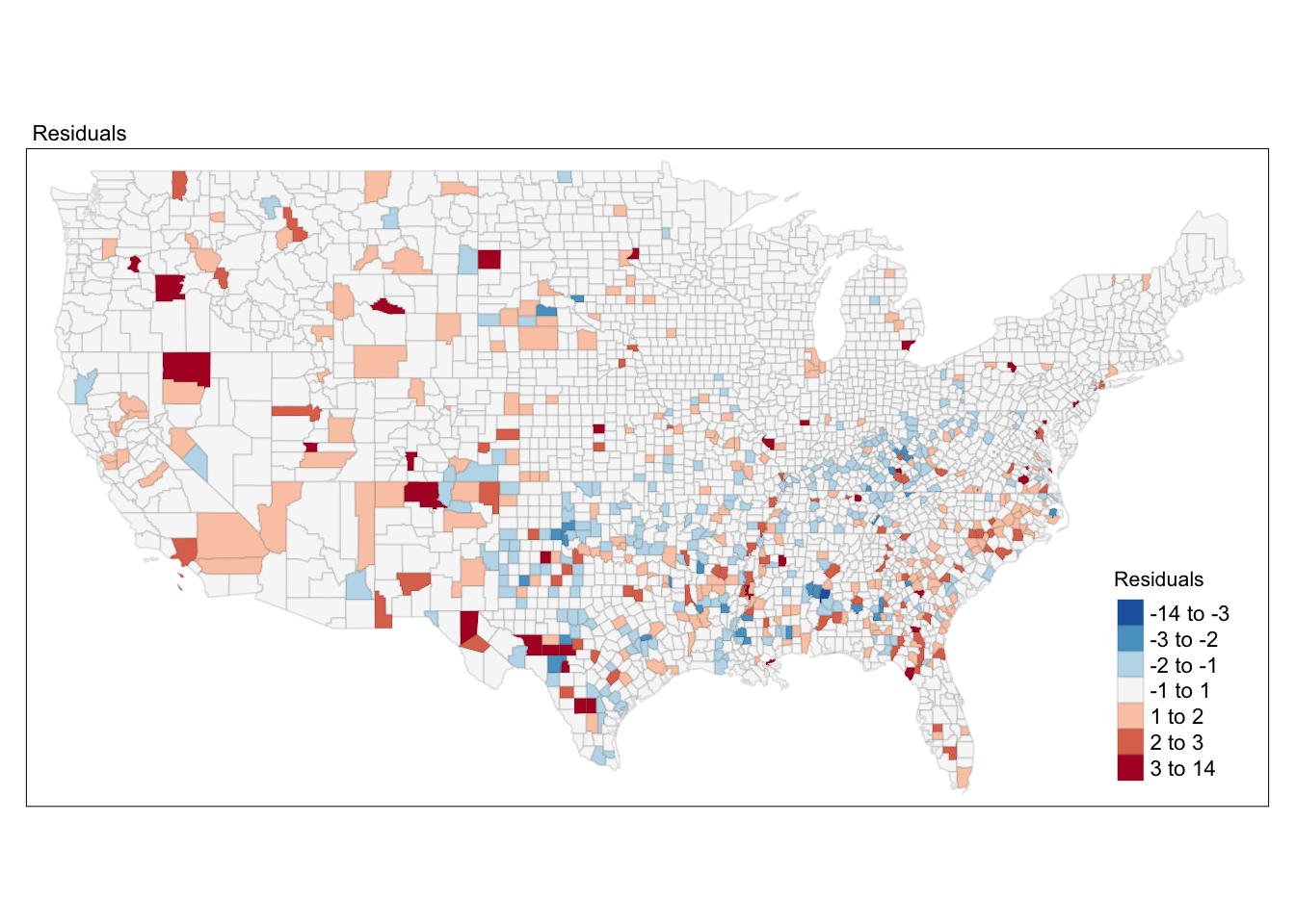
FIGURE 12.4: Map of regression model residuals
Notice the spatial patterning of areas of over-prediction (negative residuals, or blue tones) and under-prediction (positive residuals, or reddish tones). This visual inspection of the residuals is suggesting you that spatial autocorrelation in the residuals may be present here. This, however, would require a more formal test.
Remember from Chapter 9 that in order to do this first we need to turn our sf object into a sp class object and then create the spatial weight matrix. We cannot examine spatial dependence without making assumptions about the structure of the spatial relations among the units in our study. For this illustration we are going to follow Baller et al. (2001) and use 10 nearest neighbors to define the matrix to codify these spatial relations. If the code below and what it does is not clear to you, revise the notes from Chapter 9, when we first introduced it.
# We coerce the sf object into a new sp object
ncovr_sp <- as(ncovr, "Spatial")
## old-style crs object detected; please recreate object with a recent sf::st_crs()
## old-style crs object detected; please recreate object with a recent sf::st_crs()# Then we create a list of neighbours using 10 nearest neighbours criteria
xy <- coordinates(ncovr_sp)
nb_k10 <- knn2nb(knearneigh(xy, k = 10))
rwm <- nb2mat(nb_k10, style='W')
rwm <- mat2listw(rwm, style='W')We obtain the Moran’s test for regression residuals using the function lm.morantest() as below. It is important to realize that the Moran’s I test statistic for residual spatial autocorrelation takes into account the fact that the variable under consideration is a residual, computed from a regression. The usual Moran’s I test statistic does not. It is therefore incorrect to simply apply a Moran’s I test to the residuals from the regression without correcting for the fact that these are residuals.
lm.morantest(fit3_90, rwm, alternative="two.sided")##
## Global Moran I for regression residuals
##
## data:
## model: lm(formula = eq1_90, data = ncovr)
## weights: rwm
##
## Moran I statistic standard deviate = 12, p-value
## <2e-16
## alternative hypothesis: two.sided
## sample estimates:
## Observed Moran I Expectation Variance
## 9.544e-02 -1.382e-03 6.029e-05You will notice we obtain a statistically significant value for Moran’s I. If we diagnose that spatial autocorrelation is an issue, that is, that the errors (the residuals) are related systematically among themselves, then we likely have a problem and we may need to use a more appropriate approach: a spatial regression model. Before going down that road it is important to check this autocorrelation is not the result of an incorrectly specified model. It may appear when estimating a non-linear relationship with a linear model. In this scenario, Kopczewska (2021) suggests checking the remainders from the OLS estimated model on variable logarithms. It is also worth considering it may be the result of other forms of model mis-specification, such as omission of covariates or wongful inclusion of predictors.
12.5 Choosing a spatial regression model
12.5.1 The basic spatial models
If the test is significant (as in this case), then we possibly need to think of a more suitable model to represent our data: a spatial regression model. Remember spatial dependence means that (more typically) there will be areas of spatial clustering for the residuals in our regression model. So our predicted line (or hyperplane) will systematically under-predict or over-predict in areas that are close to each other. That’s not good. We want a better model that does not display any spatial clustering in the residuals.
There are two traditional general ways of incorporating spatial dependence in a regression model, through what we called a spatial error model or by means of a spatially lagged model . The Moran test doesn´t provide information to help us choose, which is why Anselin and Bera (1998) introduced the Lagrange Multiplier tests, which we will examine shortly.
The difference between these two models is both technical and conceptual. The spatial error model treats the spatial autocorrelation as a nuisance that needs to be dealt with. It includes a spatial lag of the error in the model
(lambda in the R output). A spatial error model basically implies that the:
“spatial dependence observed in our data does not reflect a truly spatial process, but merely the geographical clustering of the sources of the behaviour of interest. For example, citizens in adjoining neighbohoods may favour the same (political) candidate not because they talk to their neighbors, but because citizens with similar incomes tend to cluster geographically, and income also predicts vote choice. Such spatial dependence can be termed attributional dependence” (Darmofal 2015 p: 4)
In the example we are using the spatial error model “evaluates the extent to which the clustering of homicide rates not explained by measured independent variables can be accounted for with reference to the clustering of error terms. In this sense, it captures the spatial influence of unmeasured independent variables” (Baller et al. 2001: 567, the emphasis is ours). As Kopczewska (2021) suggests this spatial effect allows us to model “invisible or hardly measurable supra-regional characteristics, occurring more broadly than regional boundaries (e.g., cultural variables, soil fertility, weather, pollution, etc.).” (p. 218).
The spatially lagged model o spatially autoregressive model, on the other hand, incorporates spatial dependence by adding a “spatially lagged” variable \(y\) on the right hand side of our regression equation (this will be denoted as rho in the R output). Its distinctive characteristic is that it includes a spatially lagged measure of our outcome as an endogenous explanatory factor (a variable that measures the value of our outcome of interest, say crime rate, in the neighbouring areas, as defined by our spatial weight matrix). It is basically explicitly saying that the values of \(y\) in the neighbouring areas of observation \(n_i\) is an important predictor of \(y_i\) on each individual area \(n_i\) . This is one way of saying that the spatial dependence may be produced by a spatial process such as the diffusion of behaviour between neighboring units:
“If so the behaviour is likely to be highly social in nature, and understanding the interactions between interdependent units is critical to understanding the behaviour in question. For example, citizens may discuss politics across adjoining neighbours such that an increase in support for a candidate in one neighbourhood directly leads to an increase in support for the candidate in adjoining neighbourhoods”* (Darmofal 2015 p: 4).
So, in our example, what we are saying is that homicide rates in one county may be affecting the level of homicide in nearby (however we define “nearby”) counties.
As noted by Baller et al. (2001): 567:
“It is important to recognize that these models for spatial lag and spatial error processes are designed to yield indirect evidence of diffusion in cross-sectional data. However, any diffusion process ultimately requires “vectors of transmission,” i.e., identifiable mechanisms through which events in a given place at a given time influence events in another place at a later time. The spatial lag model, as such, is not able to discover these mechanisms.“ Rather, it depicts a spatial imprint at a given instant of time that would be expected to emerge if the phenomenon under investigation were to be characterized by a diffusion process. The observation of spatial effects thus indicates that further inquiry into diffusion is warranted, whereas the failure to observe such effects implies that such inquiry is likely to be unfruitful.”
A third basic model is the one that allows for autocorrelation in the predictors (Durbin factor). Here we allow for exogenous interaction effects, where the dependent variable of a given area is influenced by independent explanatory variables of other areas. In this case we include in the model a spatial lag of the predictors. These, however, have been less commonly used in practice.
These three models only have one spatial component, but this could be combined. In the last 15 years interest in models with more than one spatial component has grown. You could have models with two spatial components and even consider together the three ways of spatial interaction (in the error, in the predictors, and the dependent variable). Elhorst (2010) classified the different models according to the spatial interactions included.
| Models | Features |
|---|---|
| Manski (GNS Model) | Includes spatial lag of dependent and explatory variables, and autocorrelated errors |
| Kelejian/Prucha (SAC or SARAR Model) | Includes spatial lag of dependent model and autocorrelated errors, often call a spatial autoregressive-autoregressive model |
| Spatial Durbin Model (SDM) | Allows for spatial lag of dependent variable and explanatory variables |
| Spatial Durbin Error Model (SDEM) | Allows for lag of explanatory variables and autocorrelated errors |
| Spatial Lag Model (SAR) | The traditional spatial lag of the dependent variable model, orspatial autoregressive model |
| Spatial Error Model (SEM) | The traditional model with autocorrelated errors |
In practice, issues with overspecification mean you rarely find applications that allow for interaction at the three levels (the so-called Manski model or general nesting model, GNS for short) simultaneously. But it still useful for testing the right specification.
12.5.2 Lagrange multipliers: the bottom-up approach to select a model
The Moran’s I test statistic has high power against a range of spatial alternatives. However, it does not provide much help in terms of which alternative model would be most appropriate. Until a few years ago, the main solution was to look at a series of tests that were developed by Anselin and Bera (1998) for this purpose: the Lagrange multipliers. The Lagrange multiplier test statistics do allow a distinction between spatial error models and spatial lag models, which was the key concern before interest developed in models with more than one type of spatial effect. The Lagrange multipliers also allow to evaluate if the Kelejian/Prucha (SAC) model is appropriate. This approach, starting with a baseline OLS model, test residuals, run Lagrange multipliers, and then select the SAC or SEM model is what is referred to as the bottoms-up or specific to general approach and was the dominant workflow until recently.
Both Lagrange multiplier tests (for the error and the lagged models, LMerr and LMlag respectively), as well as their robust forms (RLMerr and RLMLag, also respectively) are included in the lm.LMtests() function. Again, a regression object and a spatial listw object must be passed as arguments. In addition, the tests must be specified as a character vector (the default is only LMerror), using the c( ) operator (concatenate), as illustrated below. Alternatively one could ask to display all tests with test="all". This would also run a test for the so called SARMA model, but Anselin advises against its use. For sparser reporting we may wrap this function within a summary() function.
summary(lm.LMtests(fit3_90, rwm, test = c("LMerr","LMlag","RLMerr","RLMlag")))## Lagrange multiplier diagnostics for spatial
## dependence
## data:
## model: lm(formula = eq1_90, data = ncovr)
## weights: rwm
##
## statistic parameter p.value
## LMerr 148.80 1 < 2e-16 ***
## LMlag 116.36 1 < 2e-16 ***
## RLMerr 35.41 1 2.7e-09 ***
## RLMlag 2.97 1 0.085 .
## ---
## Signif. codes:
## 0 '***' 0.001 '**' 0.01 '*' 0.05 '.' 0.1 ' ' 1How do we interpret the Lagrange multipliers? The interpretation of these tests focuses on their significance level. First we look at the standard multipliers (LMerr and LMlag). If both are below the .05 level, like here, this means we need to have a look at the robust version of these tests (Robust LM).
If the non-robust version is not significant, the mathematical properties of the robust tests may not hold, so we don’t look at them in those scenarios. It is fairly common to find that both the lag (LMlag) and the error (LMerr) non-robust LM are significant. If only one of them were: problem solved. We would choose a spatial lag or a spatial error model according to this (i.e., if the lag LM was significant and the error LM was not we would run a spatial lag model or viceversa). Here we see that both are significant, thus, we need to inspect their robust versions.
When we look at the robust Lagrange multipliers (RLMlag and RLMerr) here we can see only the Lagrange for the error model is significant, which suggest we need to fit a spatial error model. But there may be occasions when both are as well significant. What do we do then? Luc Anselin (2008: 199-200) proposes the following criteria:
“When both LM test statistics reject the null hypothesis, proceed to the bottom part of the graph and consider the Robust forms of the test statistics. Typically, only one of them will be significant, or one will be orders of magnitude more significant than the other (e.g., p < 0.00000 compared to p < 0.03). In that case the decision is simple: estimate the spatial regression model matching the (most) significant” robust “statistic. In the rare instance that both would be highly significant, go with the model with the largest value for the test statistic. However, in this situation, some caution is needed, since there may be other sources of misspecification. One obvious action to take is to consider the results for different spatial weight and/or change the basic (i.e., not the spatial part) specification of the model. There are also rare instances where neither of the Robust LM test statistics are significant. In those cases, more serious specification problems are likely present and those should be addressed first”.
By other specification errors Prof. Anselin refers to problems with some of the other assumptions of regression that you should be familiar with.
As noted, this way of selecting the “correct” model (the bottoms-up approach), using the Lagrange multipliers, was the most popular until about 15 years ago or so. It was attractive because it relied on observing the residuals in the non spatial model; it was computationally very efficient; and when the correct model was the spatial error or the spatial lag model simulation studies had shown it was the most effective approach (Floch and LeSaout 2018). Later we will explore other approaches. Also, since the spatial error and the spatial lag model are not nested, you could not compare them using likelihood ratio tests (Bivand, Millo, and Piras 2021).
12.6 Fitting and interpreting a spatial error model
We just saw that for the case of homicide in the 90s the bottoms up approach suggested that the spatial error model was more appropriate when using our particular definition of the spatial weight matrix. In this case then, we can run a spatial error model. Maximum likelihood estimation of the spatial error model is implemented in the spatialreg::errorsarlm() function. The formula, data set and a listw spatial weights object must be specified, as illustrated below. We are still using the 10 nearest neighbours definition. When thinking about the spatial weight matrix to use in spatial regression analysis, it is worth considering T. Smith (2009) suggestions. His work showed that highly connected matrices may result in downward bias for the coefficients when using maximum likelihood.
fit3_90_sem <- errorsarlm(eq1_90, data=ncovr, rwm)
summary(fit3_90_sem)
##
## Call:
## errorsarlm(formula = eq1_90, data = ncovr, listw = rwm)
##
## Residuals:
## Min 1Q Median 3Q Max
## -15.84281 -2.49313 -0.69615 1.60685 68.82483
##
## Type: error
## Coefficients: (asymptotic standard errors)
## Estimate Std. Error z value Pr(>|z|)
## (Intercept) 3.820725 1.147279 3.3302 0.0008677
## RD90 3.753935 0.159813 23.4895 < 2.2e-16
## PS90 1.245862 0.119091 10.4615 < 2.2e-16
## MA90 -0.044778 0.030298 -1.4779 0.1394354
## DV90 0.588880 0.062825 9.3734 < 2.2e-16
## UE90 -0.195440 0.046141 -4.2357 2.279e-05
## SOUTH_f1 2.126187 0.297569 7.1452 8.988e-13
##
## Lambda: 0.3661, LR test value: 113.9, p-value: < 2.22e-16
## Asymptotic standard error: 0.03254
## z-value: 11.25, p-value: < 2.22e-16
## Wald statistic: 126.6, p-value: < 2.22e-16
##
## Log likelihood: -9276 for error model
## ML residual variance (sigma squared): 23.62, (sigma: 4.86)
## Number of observations: 3085
## Number of parameters estimated: 9
## AIC: 18571, (AIC for lm: 18683)The spatial lag model is probably the most common specification and maybe the most generally useful way to think about spatial dependence. But we can also enter the spatial dependence as, we mentioned trough the error term in our regression equation. Whereas the spatial lag model sees the spatial dependence as substantively meaningful (in that \(y\), say homicide, in county \(i\) is influenced by homicide in its neighbours), the spatial error model simply treats the spatial dependence as capturing the effect of unobserved variables. It is beyond the scope of this introductory course to cover the mathematical details and justification of this procedure, though you can use the suggested reading (particularly the highly accessible Ward and Gleditsch (2008), book or the more recent Darmofal (2015)) or some of the other materials we discussed at the end of the chapter.
How do you interpret these results? First you need to look at the general measures of fit of the model. I know what you are thinking. Look at the R Square and compare them, right? Well, don’t. This R Square is not a real R Square, but a pseudo-R Square and therefore is not comparable to the one we obtain from the OLS regression model. Instead we can look at the Akaike Information Criterion (AIC). We can see the AIC is better for the spatial model (18571) than for the non spatial model (18683).
In this case, you can compare the regression coefficients with those from the OLS model, since we don’t have a spatial lag capturing some of their effect. Notice how one of the most notable differences is the fact that median age is no longer significant in the new model.
We are using here the 10 nearest neighbours (following the original analysis of this data), but in real practice you would need to explore whether this is the best definition and one that makes theoretical sense. Various authors, such as Chi and Zhu (2020), suggest that you would want to run the models with several specifications of the spatial weight matrix and find out how robust the findings are to various specifications. They even propose a particular method to pick up the “best” specification of the weight matrix. Kopczewska (2021) provides R code and an example of checking for sensitivity of results to various specifications of the matrix.
12.7 Fitting and interpreting a spatially lagged model
We saw that in the previous case a spatial error model was perhaps more appropriate, but we also saw earlier in one of the simpler models that there was an interaction between the variable indicating whether the county is in the South and one of the explanatory variables. This is suggestive of the kind of spatial heterogeneity we were discussing a the outset of the chapter. When the relationship of the explanatory variables is not constant across the study area we need to take this into account. Fitting the same model for the whole country may not be appropriate and there are so many interaction terms you can include before things get a difficult to interpret. A fairly crude approach, instead of adding multiple interaction terms, is to partition the data. We could, in this example, partition the data into Southern and Northern counties and run separate models for this two subsets of the data. For the next illustration, we are going to focus on the Southern countries and in a different decade, in which the lag model (as we will see) is more appropriate.
# Let´s look at southern counties
ncovr_s_sf <- subset(ncovr, SOUTH == 1)
## old-style crs object detected; please recreate object with a recent sf::st_crs()
## old-style crs object detected; please recreate object with a recent sf::st_crs()# We coerce the sf object into a new sp object
ncovr_s_sp <- as(ncovr_s_sf, "Spatial")
# Then we create a list of neighbours using 10 nearest neighbours criteria
xy_s <- coordinates(ncovr_s_sp)
nb_s_k10 <- knn2nb(knearneigh(xy_s, k = 10))
rwm_s <- nb2mat(nb_s_k10, style='W')
rwm_s <- mat2listw(rwm_s, style='W')
# We create new equation, this time excluding the southern dummy
eq2_70_S <- HR70 ~ RD70 + PS70 + MA70 + DV70 + UE70
fit4_70 <- lm(eq2_70_S, data=ncovr_s_sf)
summary(lm.LMtests(fit4_70, rwm_s, test = c("LMerr","LMlag","RLMerr","RLMlag")))## Lagrange multiplier diagnostics for spatial
## dependence
## data:
## model: lm(formula = eq2_70_S, data = ncovr_s_sf)
## weights: rwm_s
##
## statistic parameter p.value
## LMerr 1.47e+02 1 <2e-16 ***
## LMlag 1.75e+02 1 <2e-16 ***
## RLMerr 1.55e-03 1 0.97
## RLMlag 2.86e+01 1 9e-08 ***
## ---
## Signif. codes:
## 0 '***' 0.001 '**' 0.01 '*' 0.05 '.' 0.1 ' ' 1Maximum Likelihood (ML) estimation of the spatial lag model is carried out with the spatreg::lagsarlm() function. The required arguments are again a regression “formula”, a data set and a listw spatial weights object. The default method uses Ord’s eigenvalue decomposition of the spatial weights matrix.
fit4_70_sar <- lagsarlm(eq2_70_S, data=ncovr_s_sf, rwm_s)
summary(fit4_70_sar)
##
## Call:
## lagsarlm(formula = eq2_70_S, data = ncovr_s_sf, listw = rwm_s)
##
## Residuals:
## Min 1Q Median 3Q Max
## -17.13387 -4.09583 -0.95433 2.85297 65.93842
##
## Type: lag
## Coefficients: (asymptotic standard errors)
## Estimate Std. Error z value Pr(>|z|)
## (Intercept) 7.437000 1.413763 5.2604 1.437e-07
## RD70 2.247458 0.244104 9.2070 < 2.2e-16
## PS70 0.603290 0.256056 2.3561 0.018469
## MA70 -0.091496 0.041144 -2.2238 0.026160
## DV70 0.633473 0.211198 2.9994 0.002705
## UE70 -0.485272 0.099684 -4.8681 1.127e-06
##
## Rho: 0.4523, LR test value: 114.8, p-value: < 2.22e-16
## Asymptotic standard error: 0.04111
## z-value: 11, p-value: < 2.22e-16
## Wald statistic: 121, p-value: < 2.22e-16
##
## Log likelihood: -4769 for lag model
## ML residual variance (sigma squared): 49.18, (sigma: 7.013)
## Number of observations: 1412
## Number of parameters estimated: 8
## AIC: 9555, (AIC for lm: 9668)
## LM test for residual autocorrelation
## test value: 7.662, p-value: 0.0056391Remember what we said earlier in the spatial lag model we are simply adding as an additional explanatory variable the values of \(y\) in the surrounding area. What we mean by “surrounding” will be defined by our spatial weight matrix. It’s important to emphasise again that one has to think very carefully and explore appropriate definitions of “surrounding”.
In our spatial lag model you will notice that there is a new term \(Rho\). What is this? This is our spatial lag. It is a variable that measures the homicide rate in the counties that are defined as surrounding each county in our spatial weight matrix. We are simply using this variable as an additional explanatory variable to our model, so that we can appropriately take into account the spatial clustering detected by our Moran’s I test. You will notice that the estimated coefficient for this term is both positive and statistically significant. In other words, when the homicide rate in surrounding areas increases, so does the homicide rate in each country, even when we adjust for the other explanatory variables in our model.
You also see at the bottom further tests for spatial dependence, a likelihood ratio test. This is not a test for residual spatial autocorrelation after we introduce our spatial lag. What you want is for this test to be significant because in essence is further evidence that the spatial lag model is a good fit.
How about the coefficients? It may be tempting to look at the regression coefficients for the other explanatory variables for the original OLS model and compare them to those in the spatial lag model. But you should be careful when doing this. Their meaning now has changed:
“Interpreting the substantive effects of each predictor in a spatial lag model is much more complex than in a nonspatial model (or in a spatial error model) because of the presence of the spatial multiplier that links the independent variables to the dependent. In the nonspatial model, it does not matter which unit is experiencing the change on the independent variable. The effect” in the dependent variable “of a change” in the value of an independent variable “is constant across all observations” (Darmofal, 2015: 107).
Remember we say, when interpreting a regression coefficient for variable \(x_i\), that they indicate how much \(y\) goes up or down for every one unit increase in \(x_i\) when holding all other variables in the model constant. In our example, for the nonspatial model this “effect” is the same for every county in our dataset. But in the spatial lag model things are not the same. We cannot interpret the regression coefficients for the substantive predictors in the same way because the “substantive effects of the independent variables vary by observation as a result of the different neighbors for each unit in the data” (Darmofal 2015: 107).
In the standard OLS regression model, the coefficients for any of the explanatory variables measure the absolute “impact” of these variables. It is a simpler scenario. We look at the “effect” of \(x\) in \(y\) within each county. So \(x\) in county A affects \(y\) in count A. In the spatial lag model there are two components to how \(x\) affect \(y\). The predictor \(x\) affects \(y\) within each county directly but remember we are also including the spatial lag, the measure of \(y\) in the surrounding counties (call them B, C, and D). By virtues of including the spatial lag (a measure of \(y\) in county B, C and D) we are indirectly incorporating as well the “effects” that \(x\) has on \(y\) in counties B, C, and D. So the “effect” of a covariate (independent variable) is the sum of two particular “effects”: a direct, local effect of the covariate in that unit, and an indirect, spillover “effect” due to the spatial lag.
In, other words, in the spatial lag model, the coefficients only focus on the “short-run impact” of \(x_i\) on \(y_i\) , rather than the net “effect”. As Ward and Gleditsch (2008) explain “Since the value of \(y_i\) will influence the level of” homicide “in other” counties \(y_j\) and these \(y_j\) , in turn, feedback on to \(y_i\) , we need to take into account the additional effects that the short impact of \(x_i\) exerts on \(y_i\) through its impact on the level of” homicide “in other” counties. You can still read the coefficients in the same way but need to keep in mind that they are not measuring the net “effect”. Part of their “effect” will be captured by the spatial lag. Yet, you may still want to have a look at whether things change dramatically, particularly in terms of their significance (which is not the case in this example).
In sum, this implies that a change in the \(ith\) region’s predictor can affect the \(jth\) region’s outcome. We have 2 situations: (a) the direct impact of an observation’s predictor on its own outcome, and (b) the indirect impact of an observation’s neighbor’s predictor on its outcome. This leads to three quantities that we want to know:
- Average Direct Impact, which is similar to a traditional interpretation
- Average Total impact, which would be the total of direct and indirect impacts of a predictor on one’s outcome
- Average Indirect impact, which would be the average impact of one’s neighbors on one’s outcome
These quantities can be found using the impacts() function in the spdep library. We follow the example that converts the spatial weight matrix into a “sparse” matrix, and power it up using the trW() function. This follows the approximation methods described in LeSage and Pace (2009). Here, we use Monte Carlo simulation to obtain simulated distributions of the various impacts.
W <- as(rwm_s, "CsparseMatrix")
trMC <- trW(W, type="MC")
fit4_70_sar.im <- impacts(fit4_70_sar, tr=trMC, R=100)
summary(fit4_70_sar.im, zstats=TRUE, short=TRUE)
## Impact measures (lag, trace):
## Direct Indirect Total
## RD70 2.30369 1.79942 4.1031
## PS70 0.61838 0.48302 1.1014
## MA70 -0.09379 -0.07326 -0.1670
## DV70 0.64932 0.50719 1.1565
## UE70 -0.49741 -0.38853 -0.8859
## ========================================================
## Simulation results ( variance matrix):
## ========================================================
## Simulated standard errors
## Direct Indirect Total
## RD70 0.23328 0.27135 0.40515
## PS70 0.27102 0.22932 0.49148
## MA70 0.04071 0.03240 0.07195
## DV70 0.21484 0.19467 0.39866
## UE70 0.10801 0.09425 0.18968
##
## Simulated z-values:
## Direct Indirect Total
## RD70 9.776 6.664 10.092
## PS70 2.336 2.199 2.314
## MA70 -2.188 -2.165 -2.213
## DV70 3.147 2.775 3.051
## UE70 -4.541 -4.118 -4.632
##
## Simulated p-values:
## Direct Indirect Total
## RD70 < 2e-16 2.7e-11 < 2e-16
## PS70 0.0195 0.0279 0.0207
## MA70 0.0287 0.0304 0.0269
## DV70 0.0017 0.0055 0.0023
## UE70 5.6e-06 3.8e-05 3.6e-06We see that all the variables have significant direct, indirect and total effects. You may want to have a look at how things differ when you just run a non spatial model.
12.8 Beyond the SAR and SEM models
Given the “galaxy” of spatial models, newer approaches to select the one to run have been proposed. LeSage and Pace (2009) proposes a top-down approach that involved starting with the spatial Durbin model (SDM) and based on likelihood ratio tests to select the best model. Elhorst (2010), on the other hand, proposes to start with the OLS model, run the Lagrange multipliers, and then run a likelihood ratio test to see if the spatial Durbin model would be more appropriate. Why the Durbin model? Why not Manski or the SAR model? Elhorst (2010) corroborates that the Manski model can be estimated but the parameters cannot be interpreted in a meaningful way (the endogenous and exogenous effects cannot be distinguished from each other) and the SAR or Kelejian/Prucha model “will suffer from omitted variables bias if the true data-generation process is a spatial Durbin or a spatial Durbin error model” and that similarly the same happens for the spatial Durbin error model” (p. 14).
If you paid attention the summary of the lag model we ran in the previous section included at the bottom a test for remaining residual spatial autocorrelation. This means our model is still not filtering all the spatial dependency that is present here. Perhaps here, and following the workflow proposed by Elhorst (2010), we need to consider if the spatial Durbin model (SDM) would be more appropriate. We can run this model and then contrast it with the SAR model.
fit4_70_sdm <- lagsarlm(eq2_70_S, data=ncovr_s_sf, rwm_s, Durbin = TRUE,
                        method ="LU")
summary(fit4_70_sdm)
##
## Call:
## lagsarlm(formula = eq2_70_S, data = ncovr_s_sf, listw = rwm_s,
## Durbin = TRUE, method = "LU")
##
## Residuals:
## Min 1Q Median 3Q Max
## -18.09108 -4.13069 -0.88963 2.84179 67.03240
##
## Type: mixed
## Coefficients: (asymptotic standard errors)
## Estimate Std. Error z value Pr(>|z|)
## (Intercept) 9.996665 2.080609 4.8047 1.550e-06
## RD70 2.266521 0.350632 6.4641 1.019e-10
## PS70 0.297629 0.312080 0.9537 0.3402394
## MA70 -0.066899 0.055596 -1.2033 0.2288603
## DV70 0.819995 0.244796 3.3497 0.0008090
## UE70 -0.185133 0.129563 -1.4289 0.1530326
## lag.RD70 0.262121 0.515226 0.5087 0.6109276
## lag.PS70 1.071509 0.518284 2.0674 0.0386949
## lag.MA70 -0.023245 0.088356 -0.2631 0.7924840
## lag.DV70 -0.414450 0.429808 -0.9643 0.3349117
## lag.UE70 -0.737893 0.202560 -3.6428 0.0002697
##
## Rho: 0.415, LR test value: 79.91, p-value: < 2.22e-16
## Asymptotic standard error: 0.04542
## z-value: 9.138, p-value: < 2.22e-16
## Wald statistic: 83.5, p-value: < 2.22e-16
##
## Log likelihood: -4759 for mixed model
## ML residual variance (sigma squared): 48.66, (sigma: 6.976)
## Number of observations: 1412
## Number of parameters estimated: 13
## AIC: 9544, (AIC for lm: 9622)
## LM test for residual autocorrelation
## test value: 13.98, p-value: 0.00018426We can then compare the nested models using information criteria with `AIC() and BIC(). Using this information criteria, we choose the model with the lowest AIC and BIC.
output_1 <- AIC(fit4_70, fit4_70_sar, fit4_70_sdm)
output_2 <- BIC(fit4_70, fit4_70_sar, fit4_70_sdm)
table_1 <- cbind(output_1, output_2)
table_1
## df AIC df BIC
## fit4_70 7 9668 7 9704
## fit4_70_sar 8 9555 8 9597
## fit4_70_sdm 13 9544 13 9613Our results indicate that AIC favours the SDM model whereas the BIC favours the simpler SAR model. We can also run a likelihood ratio test to compare the two spatial nested models using spatialreg::LR.Sarlm() (that deprecates spded::LR.sarlm() you may still see mentioned in other textbooks). Here we look for the model with the highest log likelihood:
LR.Sarlm(fit4_70_sdm, fit4_70_sar)##
## Likelihood ratio for spatial linear models
##
## data:
## Likelihood ratio = 21, df = 5, p-value = 0.001
## sample estimates:
## Log likelihood of fit4_70_sdm
## -4759
## Log likelihood of fit4_70_sar
## -4769The LR test is significant suggesting we should favour the spatial Durbin model. If it had been insignificant we would have had to choose the more parsimonious model.
As with the spatial lag model, here we need to be careful when interpreting the regression coefficients. We also need to estimate the “impacts” in a similar manner we illustrated above.
fit4_70_sdm.im <- impacts(fit4_70_sdm, tr=trMC, R=100)
summary(fit4_70_sdm.im, zstats=TRUE, short=TRUE)
## Impact measures (mixed, trace):
## Direct Indirect Total
## RD70 2.3255 1.99733 4.3228
## PS70 0.3562 1.98440 2.3406
## MA70 -0.0694 -0.08471 -0.1541
## DV70 0.8164 -0.12307 0.6933
## UE70 -0.2251 -1.35289 -1.5779
## ========================================================
## Simulation results ( variance matrix):
## ========================================================
## Simulated standard errors
## Direct Indirect Total
## RD70 0.29855 0.6440 0.6312
## PS70 0.28645 0.7654 0.7383
## MA70 0.05711 0.1296 0.1137
## DV70 0.26395 0.6772 0.6877
## UE70 0.12024 0.2851 0.2694
##
## Simulated z-values:
## Direct Indirect Total
## RD70 7.681 3.1783 6.875
## PS70 1.243 2.6410 3.220
## MA70 -1.267 -0.6544 -1.382
## DV70 3.269 -0.2063 1.052
## UE70 -1.856 -4.8483 -5.961
##
## Simulated p-values:
## Direct Indirect Total
## RD70 1.6e-14 0.0015 6.2e-12
## PS70 0.2140 0.0083 0.0013
## MA70 0.2053 0.5129 0.1671
## DV70 0.0011 0.8366 0.2930
## UE70 0.0634 1.2e-06 2.5e-09Notice how in this model only three inputs remain significant, resource deprivation, population structure, and unemployment. The sign of the coefficients remain the same for all the inputs. In most circumstances we see that when the direct effect is positive the indirect effect is also positive, and when the direct is negative the indirect is negative. Only for the insignificant effect of divorce we see a positive direct effect and a negative indirect effect.
As suggested by Kopczewska (2021), we can also examine the proportion of the direct effect in the total effect:
direct <- fit4_70_sdm.im$res$direct
indirect <- fit4_70_sdm.im$res$indirect
total <- fit4_70_sdm.im$res$total
direct/total
## RD70 PS70 MA70 DV70 UE70
## 0.5380 0.1522 0.4503 1.1775 0.1426The proportion of the (significant) direct effect ranges from 14% (for unemployment), fairly marginal, to 54% (for resource deprivation), about half of it. Another way of looking at it is by relation of the direct to the indirect effect by looking at its ratio in absolute values:
abs(direct)/abs(indirect)## RD70 PS70 MA70 DV70 UE70
## 1.1643 0.1795 0.8193 6.6332 0.1663When the ratio is greater than 1 this suggest that the direct effect prevails, as we see for resource deprivation. With a score lower than 1 this indicates that the spillover effect is greater than that of internalisation as we see for population structure and unemployment.
12.9 Summary and further reading
This chapter has introduced some of the issues associated with spatial regression. We have deliberately avoided mathematical detail and focused instead on providing a general and more superficial introduction of some of the issues associated with fitting, choosing, and interpreting basic spatial regression models in R. We have also favoured the kind of models that have been previously discussed in the criminological literature, those relying on the frequentist tradition, use of maximum likelihood, simultaneous autoregressive models, and the incorporation of the spatial structure through a neighbourhood matrix. These are not the only ways of fitting spatial regression, though. The functions of spatialreg, for example, allow for newer generalized method of moments (GMM) estimators. On the other hand, other scientific fields have emphasised conditional autoregressive models (see Wall (2004) for the difference between CAR and SAR) and there is too a greater reliance, for example in spatial epidemiology, on Bayesian approaches. Equally we have only focused on cross sectional models, without any panel or spatio-temporal dimension to them. As Ralph Sockman was attributed to say “the larger the island of knowledge, the longer the shoreline of wonder”. Learning more about spatial analysis only leads to discovering there is much more to learn. This chapter mostly aims to make you realise this about spatial regression and hopefully tempt you into wanting to continue this journey. In what follows we offer suggestions for this path.
There are a number of accessible, if somehow dated, introductory discussions of spatial regression for criminologists: Tita and Radil (2010) and Bernasco and Elffers (2010). The books by Ward and Gleditsch (2008), Darmofal (2015), and Chi and Zhu (2020) expand this treatment with the social student in mind. Pitched at a similar level is Anselin and Rey (2014). More mathematically detailed treatment and a wider diversity of models, including those appropriate for panel data, is provided in several spatial econometric books such as LeSage and Pace (2009), Elhorst (2014) or Kelejian and Piras (2017). In these econometric books you will also find more details about a newer approaches to estimation, such as GMM. If you are interested in exploring the Bayesian approach to modeling spatial lattice data, we suggest you start with Haining and Li (2020).
There are also a number of resources that focus on R capabilities for spatial regression and that have inspired our writing. It is important to highlight that many of these, even the more recent ones, do not account properly for how spatialreg has deprecated the regression functionality of spdep, even if they still provide useful instruction (for the basic architecture of the functions that have migrated to spatialreg has not being started from scratch). Anselin (2007) workbook offers a detailed explanation of the spatial regression capabilities through spdep, most of which is still transferable to the equivalent functions in spatialreg. This workbook indeed uses the “ncovr” dataset and may be a useful continuation point for what we have introduced here. Kopczewska (2021) provides one of the most up to date discussions of spatial regression with R also pitched at a level the reader of this book should find accessible. Bivand, Millo, and Piras (2021) offers a more technical, up to date, and systematic review of the evolution of the software available for spatial econometrics in R. It is definitely a must read. For Bayesian approaches to spatial regression using R, which we have not had the space to cover in this volume, we recommend Lawson (2021a), Lawson (2021c), Gomez-Rubio, Ferrandiz, and Lopez (2005), and Blangiardo and Cameletii (2015), all with a focus on health data.
Aside from these reading resources, there are two series of lectures available in YouTube that provide good introductions to the field of spatial econometric. Prof. Mark Burkey spatial econometric reboot and Luc Anselin lectures in the GeoDa Software channel.
Although the focus of this chapter has been on spatial regression, there are other approaches that are used within crime analysis for the purpose of predicting crime a particular areas such as risk terrain modeling or the use of other machine learning algorithms for prediction purposes. Those are well beyond the scope of this book. Risk terrain modeling (Caplan and Kennedy 2016) is generally actioned through the RTDMx sofware commercialised by its proponents. In a recent paper Wheeler and Steenbeek (2021) illustrate how random forest, a popular machine learning algorithm, can also be used to generate crime predictions at micro places. Dr. Gio Circo is currently developing a package (quickGrid) to apply the methods proposed by Wheeler and Steenbeek (2021).